My notes for Week 1 of the Natural Language Processing with Attention Labels Course in the Natural Language Processing Specialization Offered by DeepLearning.AI on Coursera
- Seq2Seq models are used for Neural Machine Translation (NMT) tasks.
- Attention mechanisms help the model focus on different parts of the input sequence during translation.
- BLEU and ROUGE are evaluation metrics for NMT.
- Decoding methods like Beam Search and Minimum Bayes Risk help generate translations.
Intro
This course covers most modern practical NLP methods. We’ll use a powerful technique called attention to build several different models. Some of the things we build using the attention mechanism, include a powerful language translation model, an algorithm capable of summarizing texts, a model that can actually answer questions about the piece of text, and a chat bot that we can actually have a conversation with.
We also take another look at sentiment analysis.
When it comes to modern deep learning, there’s a sort of new normal, which is to say, most people aren’t actually building and training models from scratch. Instead, it’s more common to download a pre-trained model and then tweak it and find units for your specific use case. In this course, we show we how to build the models from scratch, but we also provide we custom pre-trained models that we created just for you. By training them continuously for weeks on the most powerful TPU clusters that are currently only available to researchers as Google.
Seq2Seq
Outline:
- Introduction to Neural Machine Translation
- Seq2Seq model and its shortcomings
- Solution for the information bottleneck
The sequential nature of models we learned in the previous course (RNNs, LSTMs, GRUs) does not allow for speed ups within training examples, which becomes critical at longer sequence lengths, as memory constraints limit batching across examples. (because we can run different batches or examples in parallel or even different directions)

In other words, if we rely on sequences and we need to know the beginning of a text before being able to compute something about the ending of it, then we can not use parallel computing. We would have to wait until the initial computations are complete. This isn’t good, because if your text is too long, then
- It’ll take a long time for we to process it and
- There is the information loss mentioned earlier in the text as we approach the end.
Seq2Seq model
- Introduced by Google in 2014
- Maps variable-length sequences to fixed-length memory
- LSTMs and GRUs are typically used to overcome the vanishing gradient problem
Therefore, attention mechanisms have become critical for sequence modeling in various tasks, allowing modeling of dependencies without caring too much about their distance in the input or output sequences.
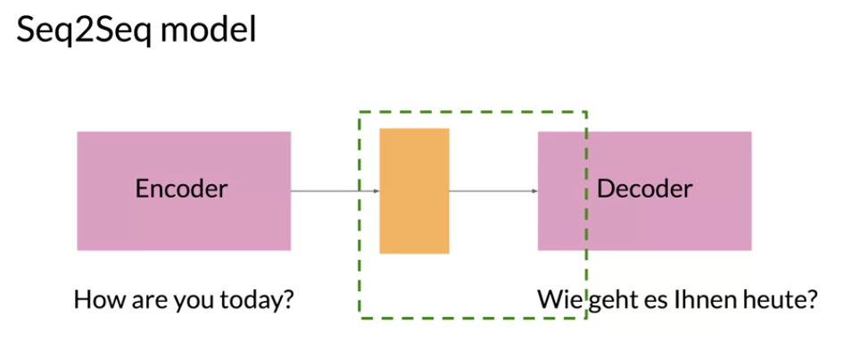
in this encoder decoder architecture the yellow block in the middle is the final hidden state produced by the encoder. It’s essentials a compressed representation of the sequence in this case the English sentence. The problem with RNN is they tend to have a bias for representing more recent data.
One approach to overcome this issue is to provide the decoder with the attention layer.
3: Alignment
Alignment is an old problem and there are a number of papers on learning to align and translate which helped put attention mechanism into focus.
- NEURAL MACHINE TRANSLATION BY JOINTLY LEARNING TO ALIGN AND TRANSLATE 2016
- Jointly Learning to Align and Translate with Transformer Models 2019
berliner = citizen of berlin
berliner = jelly doughnut
Not all words translate precisely to another word. Adding an attention layers allows the model to give different words more importance when translating another word. This is a good task for an attention layer
Developing intuition about alignment:
also check out this page Deep Learning: The Good, the Bad and the Ugly in a 2017 talk, Lukasz Kaiser referred to [K,V] as a memory. We want to manage information better in our model. We keep the information in a memory consisting of keys and values. (It needs to be differentiable so we can use it with back propagation)
Then we put in the query a sequence and in the keys another sequence (depending on the task they may be the same say for summarization or different for alignment or translation) By combining Q K using a Softmax we get a vector of probabilities each position in the memory is relevant. weight matrix to apply to the values in the memory.
- get all of the available hidden states ready for the encoder and do the same for the first hidden states of the decoder. (In the example, there are two encoder hidden states, shown by blue dots, and one decoder hidden states.)
- Next, score each of the encoder hidden states by getting its dot product between each encoder state and decoder hidden states.
A higher score means that the hidden state has greater influence on the output.
Then we run the scores through a Softmax, squashing them between 0 and 1, and giving the attention distribution.
- Take each encoder hidden state, and multiply it by its Softmax score, which is a number between 0 and 1, this results in the alignments vector.
- Add up everything in the alignments vector to arrive at what’s called the context vector.
Attention
The attention mechanism uses encoded representations of both the input or the encoder hidden states and the outputs or the decoder hidden states. The keys and values are pairs. Both of dimension NN, where NN is the input sequence length and comes from the encoder hidden states. Keys and values have their own respective matrices, but the matrices have the same shape and are often the same. While the queries come from the decoder hidden states. One way we can think of it is as follows. Imagine that we are translating English into German. We can represent the word embeddings in the English language as keys and values. The queries will then be the German equivalent. We can then calculate the dot product between the query and the key. Note that similar vectors have higher dot products and non-similar vectors will have lower dot products. The intuition here is that we want to identify the corresponding words in the queries that are similar to the keys. This would allow your model to “look” or focus on the right place when translating each word.
We then run a Softmax:
softmax(QK^T ) \tag{1}
That gives a distribution of numbers between 0 and 1.
We then would multiply the output by V. Remember V in this example was the same as our keys, corresponding to the English word embeddings. Hence the equation becomes
softmax(QK^T )V {#sec-softmax-formula-2}
In the matrix, the lighter square shows where the model is actually looking when making the translation of that word. This mapping isn’t necessarily be one to one. The lighting just tells we to what extent is each word contributing to the input that’s fed into the decoder. As we can see several words can contribute to translating another word, depending on the weights (output) of the softmax that we use to create the new input. a picture of attention in translation with English to German An important thing to keep in mind is that the model should be flexible enough to connect each English word with its relevant German word, even if they don’t appear in the same position in their respective sentences. In other words, it should be flexible enough to handle differences in grammar and word ordering in different languages.
In a situation like the one just mentioned, where the grammar of foreign language requires a difference word order than the other, the attention is so flexible enough to find the connection. The first four tokens, the agreements on the, are pretty straightforward, but then the grammatical structure between French and English changes. Now instead of looking at the corresponding fifth token to translate the French word zone, the attention knows to look further down at the eighth token, which corresponds to the English word area, glorious and necessary. It’s pretty amazing, was a little matrix multiplication can do.
So attention is a layer of calculations that let your model focus on the most important parts of the sequence for each step. Queries, values, and keys are representations of the encoder and decoder hidden states. And they’re used to retrieve information inside the attention layer by calculating the similarity between the decoder queries and the encoder key- value pairs.
Evaluation metrics for Machine Translation
BLEU
- The authors of (Papineni et al. 2002) introduced the BLEU score.
- The closer the BLEU score is to 1, the better a model preforms.
- The closer to 0, the worse it does.
To get the BLEU score, the candidates and the references are usually based on an average of unigrams, bigrams, trigrams or even four-gram precision. For example using uni-grams:
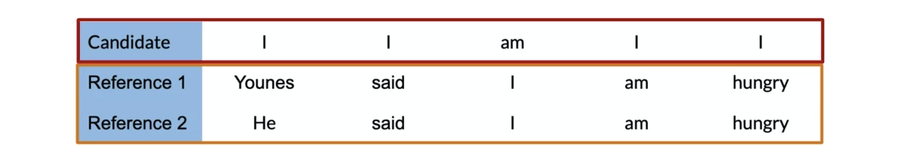
We would sum over the unique n-gram counts in the candidate and divide by the total number of words in the candidate. The same concept could apply to unigrams, bigrams, etc. One issue with the BLEU score is that it doesn’t take into account semantics, so it doesn’t take into account the order of the n-grams in the sentence.
BLEU = BP\Bigl(\prod_{i=1}^{4}\text{precision}_i\Bigr)^{(1/4)} \tag{2}
with the Brevity Penalty and precision defined as:
BP = min\Bigl(1, e^{(1-({ref}/{cand}))}\Bigr) \tag{3}
\text{Precision}_i = \frac {\sum_{snt \in{cand}}\sum_{i\in{snt}}min\Bigl(m^{i}_{cand}, m^{i}_{ref}\Bigr)}{w^{i}_{t}} \tag{4}
where:
- m^{i}_{cand}, is the count of i-gram in candidate matching the reference translation.
- m^{i}_{ref}, is the count of i-gram in the reference translation.
- w^{i}_{t}, is the total number of i-grams in candidate translation.
ROUGE
(Lin 2004) introduced a similar method for evaluation called the ROUGE score which calculates precision and recall for machine texts by counting the n-gram overlap between the machine texts and a reference text. Here is an example that calculates recall:
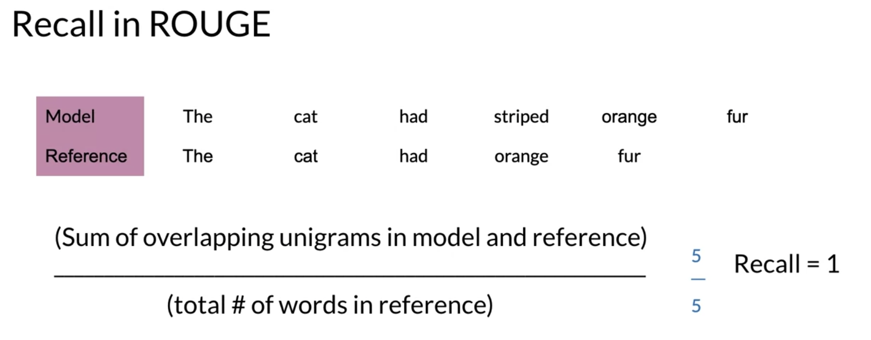
Rouge_{recall} = \sum \frac{(\{\text{prediction n-grams}\} \cap \{ \text{test n-grams}\})}{\vert{ \text{test n-grams}}\vert } \tag{5}
Rouge also allows we to compute precision as follows:
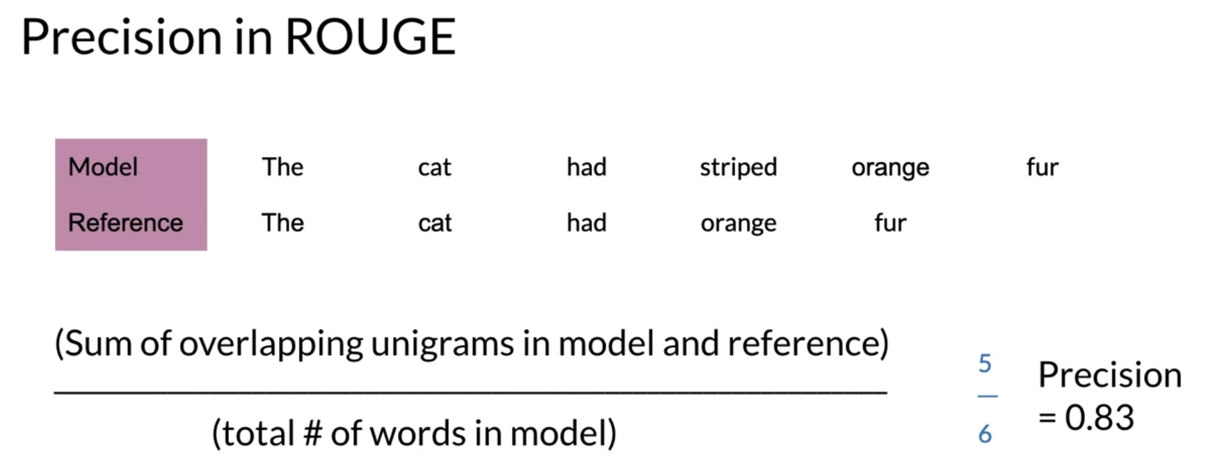
\text{ROUGE}_{\text{precision}} = \sum \frac{(\{\text{prediction n-grams}\} \cap \{ \text{test ngrams}\})}{\vert\{ \text{vocab}\}\vert} \tag{6}
The ROUGE-N refers to the overlap of N-grams between the actual system and the reference summaries. The F-score metric combines Recall and precision into one metric.
F_{score}= 2 \times \frac{(\text{precision} \times \text{recall})}{(\text{precision} + \text{recall})} \tag{7}
Decoding
Random sampling
Random sampling for decoding involves drawing a word from the softmax distribution. To explore the latent space it is possible to introduce a temperature variable which controls the randomness of the sample.
def logsoftmax_sample(log_probs, temperature=1.0):
  """Returns a sample from a log-softmax output, with temperature.
  Args:
    log_probs: Logarithms of probabilities (often coming from LogSofmax)
    temperature: For scaling before sampling (1.0 = default, 0.0 = pick argmax)
  """
  # This is equivalent to sampling from a softmax with temperature.
  u = np.random.uniform(low=1e-6, high=1.0 - 1e-6, size=log_probs.shape)
  g = -np.log(-np.log(u))
  return np.argmax(log_probs + g * temperature, axis=-1)
Beam Search
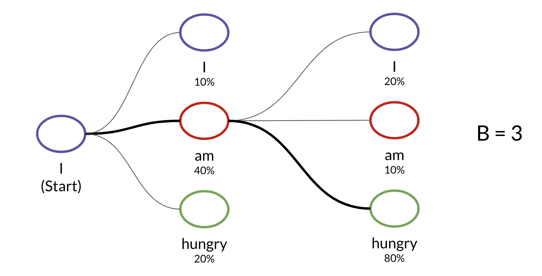
The beam search algorithm is a limited (best-first search). The parameter for the beam width limits the choices considered at each step.
Minimum Bayes Risk
MBR (Minimum Bayes Risk) Compares many samples against one another. To implement MBR:
- Generate several random samples.
- Compare each sample against all the others and assign a similarity score using ROUGE.
- Select the sample with the highest similarity: the golden one.
Summary
- Maximal Probability is a baseline - but not a particularly good one when the data is noisy.
- Random sampling with temperature is better.
- Beam search uses conditional probabilities and the parameter.
- MBR takes several samples and compares them against each other to find the golden one.
note: although not mentioned in the next week’s notes Beam Search is useful for improving the summarization task. We can extract a golden summary from a number of samples using MBR. ROUGE-N is the preferred metric for evaluating summarization
References
- - (Peters et al. 2018)
- (Alammar 2024)
Citation
@online{bochman2021,
  author = {Bochman, Oren},
  title = {Neural {Machine} {Translation}},
  date = {2021-03-20},
  url = {https://orenbochman.github.io/notes-nlp/notes/c4w1/},
  langid = {en}
}