My notes for Week 3 of the Natural Language Processing with Sequence Models Course in the Natural Language Processing Specialization Offered by DeepLearning.AI on Coursera
- Vanishing gradients
- Named entity recognition
- LSTMs
- Feature extraction
- Part-of-speech tagging
- Data generators
RNNs and Vanishing Gradients
Advantages of RNNs RNNs allow us to capture dependancies within a short range and they take up less RAM than other n-gram models.
Disadvantages of RNNs RNNs struggle with longer term dependencies and are very prone to vanishing or exploding gradients.
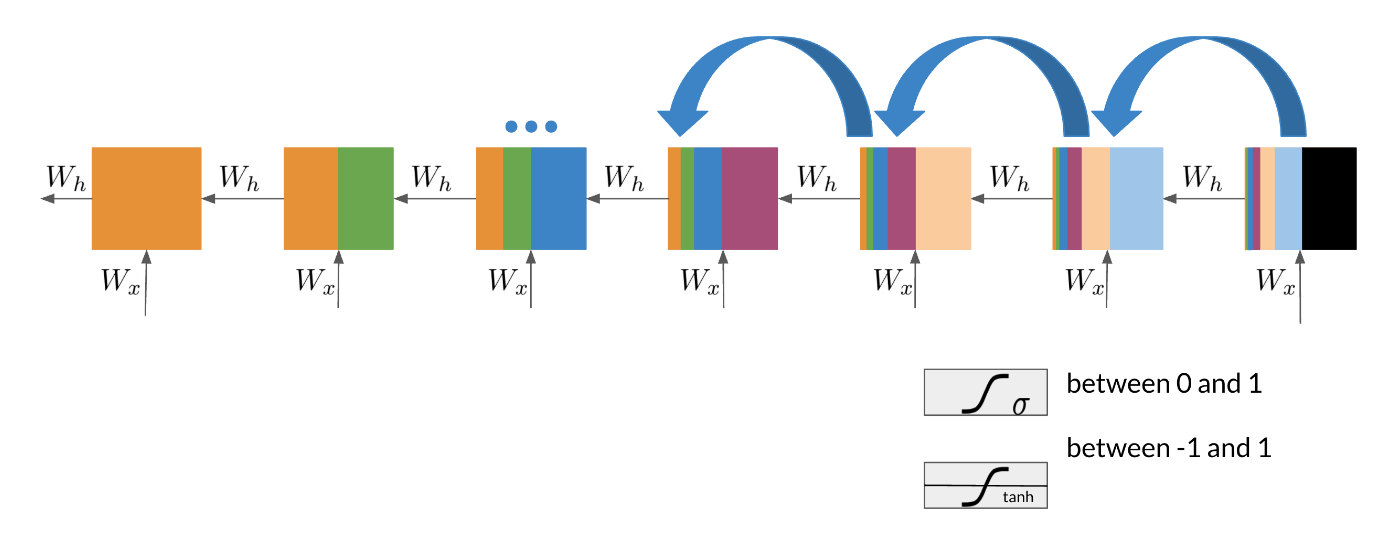
Note that as we are back-propagating through time, we end up getting the following:
Note that the sigmoid and tanh functions are bounded by 0 and 1 and -1 and 1 respectively. This eventually leads us to a problem. If we have many numbers that are less than |1|, then as we go through many layers, and we take the product of those numbers, we eventually end up getting a gradient that is very close to 0. This introduces the problem of vanishing gradients.
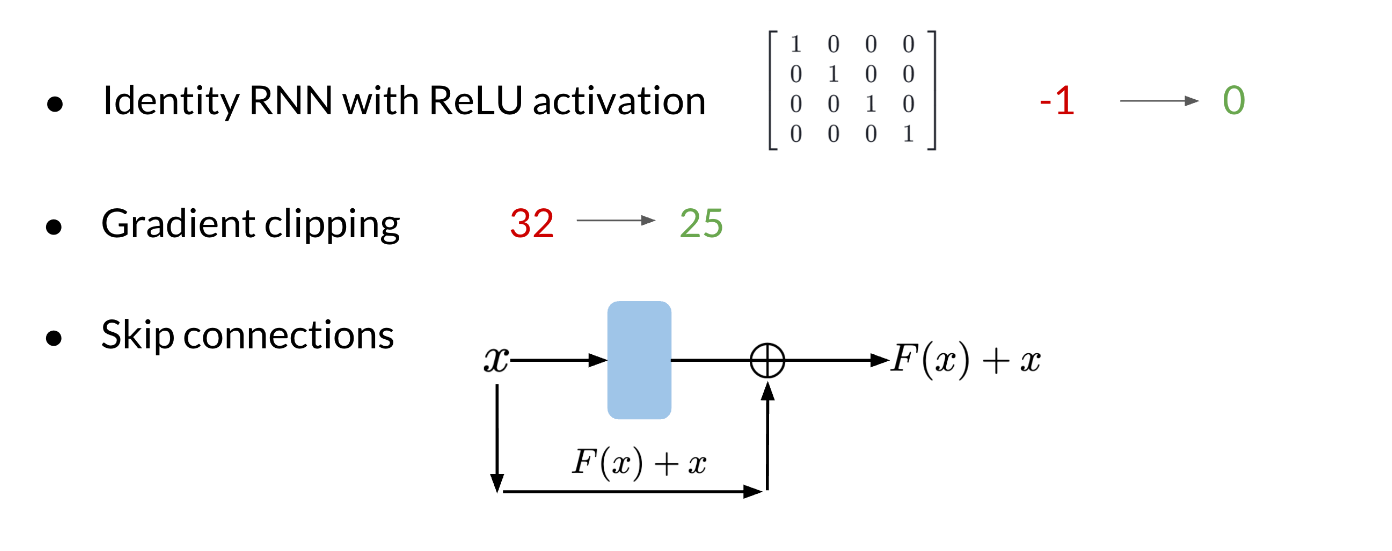
Solutions to Vanishing Gradient Problems
(Optional) Intro to optimization in deep learning: Gradient Descent
Check out this blog from Paperspace.io if you’re interested in understanding in more depth some of the challenges in gradient descent.
Lab: Lecture Notebook: Vanishing Gradients
Introduction to LSTMs
The LSTM allows your model to remember and forget certain inputs. It consists of a cell state and a hidden state with three gates. The gates allow the gradients to flow unchanged. We can think of the three gates as follows:
Input gate: tells we how much information to input at any time point.
Forget gate: tells we how much information to forget at any time point.
Output gate: tells we how much information to pass over at any time point.
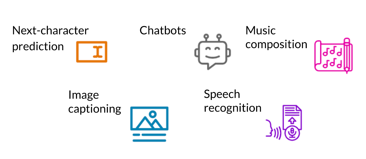
There are many applications we can use LSTMs for, such as:
(Optional) Understanding LSTMs
Here’s a classic post on LSTMs with intuitive explanations and diagrams, to complement this week’s material.
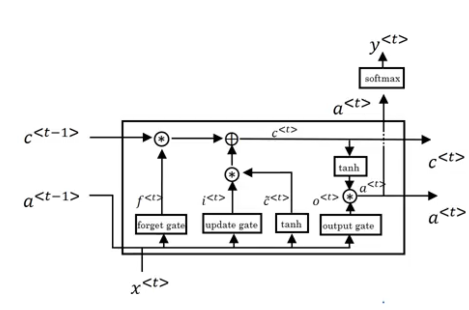
LSTM Architecture
The LSTM architecture could get complicated and don’t worry about it if we do not understand it. I personally prefer looking at the equation, but I will try to give we a visualization for now and later this week we will take a look at the equations.
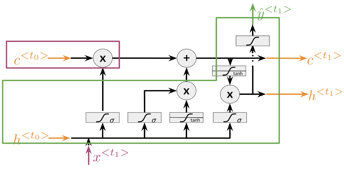
Note that there is the cell state and the hidden state, and then there is the output state. The forget gate is the first activation in the drawing above. It makes use of the previous hidden state h^{<t_0>} and the input x^{<t_0>}. The input gate makes use of the next two activations, the sigmoid and the tanh. Finally the output gate makes use of the last activation and the tanh right above it. This is just an overview of the architecture, we will dive into the details once we introduce the equations.
Introduction to Named Entity Recognition
Named Entity Recognition (NER) locates and extracts predefined entities from text. It allows we to find places, organizations, names, time and dates. Here is an example of the model we will be building:
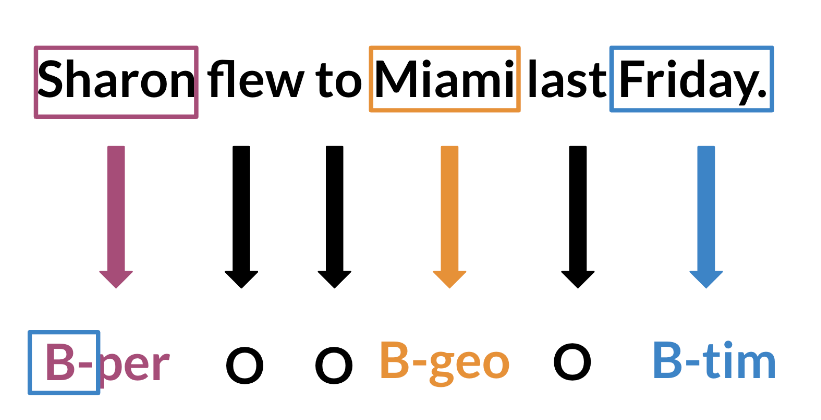
NER systems are being used in search efficiency, recommendation engines, customer service, automatic trading, and many more.
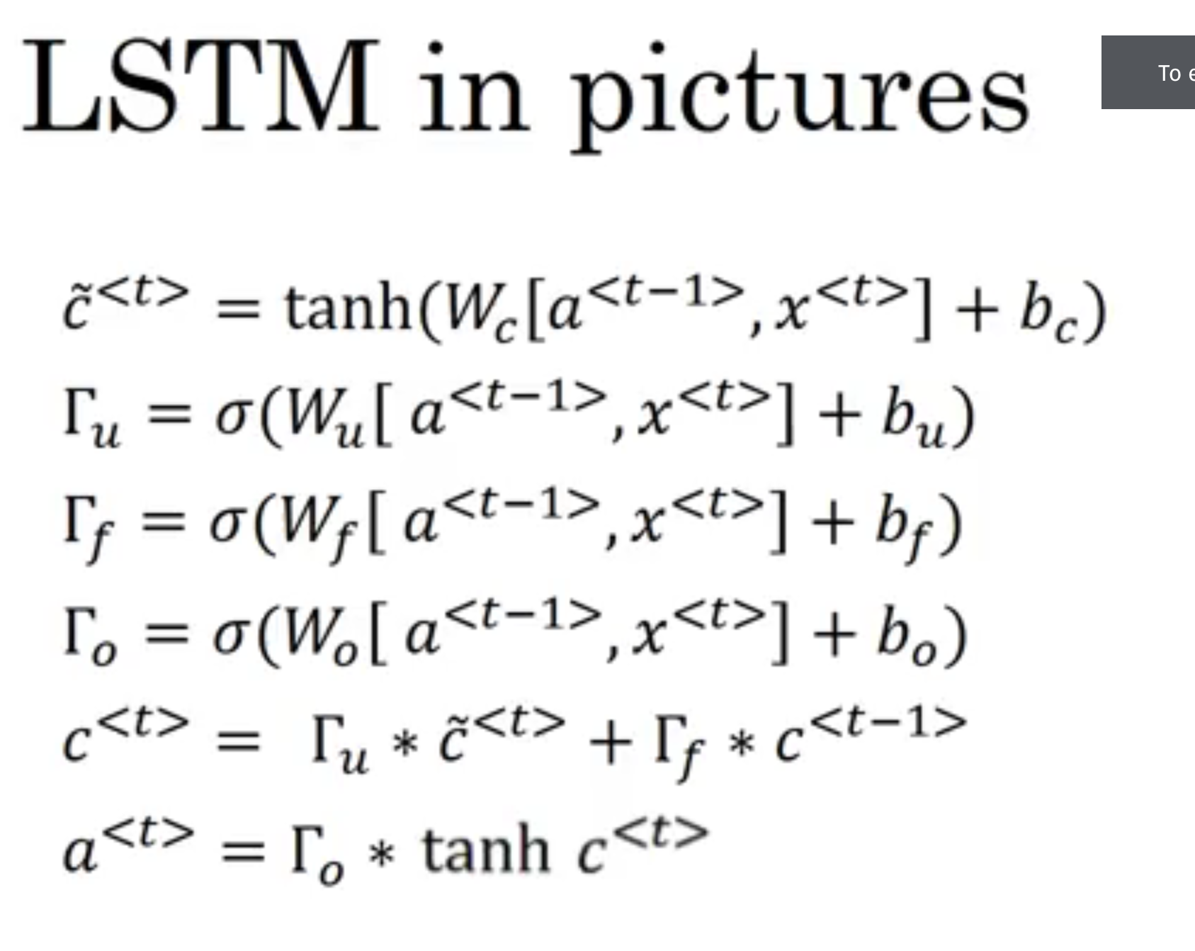
LSTM equations (Optional)
These are the LSTM equations related to the gates I had previously spoken about:
f = \sigma(W_f[h_{t-1}; x_t] + b_f) \qquad \text{Forget} \tag{1}
i = \sigma(W_i[h_{t-1}; x_t] + b_i) \qquad \text{Input} \tag{2}
g = \tanh(W_g[h_{t-1}; x_t] + b_g) \qquad \text{Gate} \tag{3}
c_t = f \odot c_{t-1} + i \odot g \qquad \text{Cell State} \tag{4}
o = \sigma(W_o[h_{t-1}; x_t] + b_o) \qquad \text{Output} \tag{5}
We can think of:
- The forget gate as a gate that tells we how much information to forget,
- The input gate, tells we how much information to pick up.
- The gate gate as the gate containing information. This is multiplied by the input gate (which tells we how much of that information to keep).
Training NERs: Data Processing
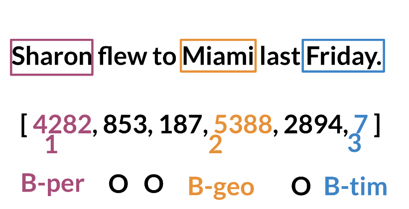
Processing data is one of the most important tasks when training AI algorithms. For NER, we have to:
Convert words and entity classes into arrays:
Pad with tokens: Set sequence length to a certain number and use the
token to fill empty spaces Create a data generator:
Once we have that, we can assign each class a number, and each word a number.
Training an NER system:
- Create a tensor for each input and its corresponding number
- Put them in a batch ==> 64, 128, 256, 512 …
- Feed it into an LSTM unit
- Run the output through a dense layer
- Predict using a log softmax over K classes
Here is an example of the architecture:
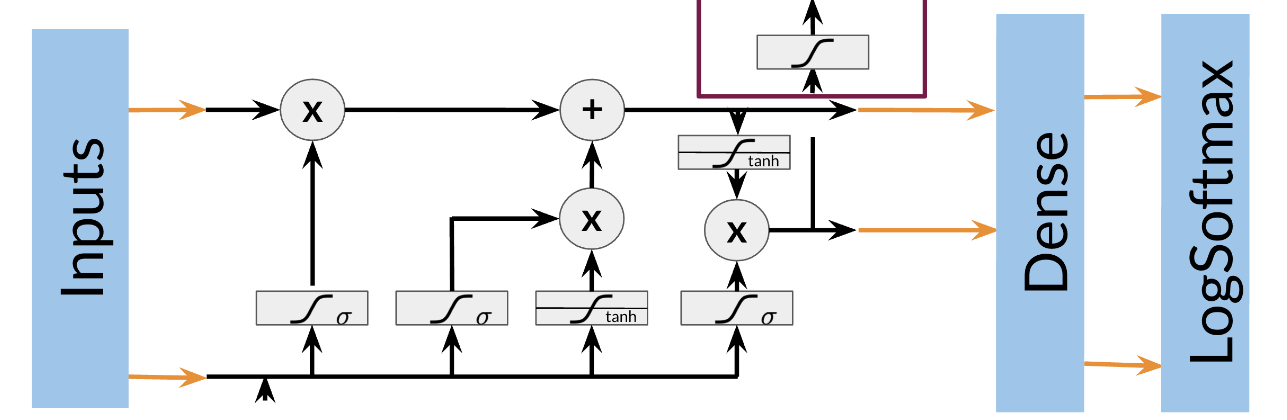
Note that this is just one example of an NER system. Different architectures are possible.
Long Short-Term Memory (Deep Learning Specialization C5)
Note: this section is based on a transcript of the video from the Deep Learning Specialization.
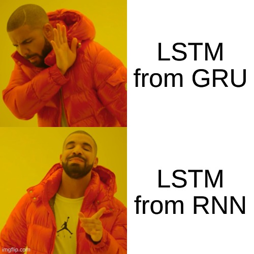
In this video Andrew Ng explains the Long Short-Term Memory (LSTM) as if it was developed from the GRU rather than RNNs. Sure the GRU has one less equation but its just about as complicated as the LSTM … The people who came up with it had 20 years to understand LSTM before they figured these out. We on the other hand have covered neither RNNs not GRUs and have none of that intuition they provide.
LSTM also have a number of variations, such as the peephole connection, the carousal connection, and the coupled forget and input gates. 😱
In the other course on Deep Learning, Ng builds things up using a number of videos starting with notation. RNNs, different types of RNNs, and then the LSTM. The vanishing gradient problem with RNN and then the GRUs.
I find the notation used very annoying but at least it is explained in the other course and seems to be motivated by time series. In Rnns we process the data in two dimensions. One is for the sequence index used in the super script. The other is for applying multiple layers which we don’t seem to consider.
Rnns learn weights more weights as the sequence grows and though not clear these weights are shared across the RNN units.
X^{(i)<t>} is the input at time t for the ith example.
y^{(i)<t>} is the output at time t for the ith example.
T_x^{(i)} is the length of the input sequence for the ith example.
T_y^{(i)} is the length of the output sequence for the ith example.
is $T_x^(i) = T_y^(i) not necessarily. (e.g. translation can be longer or shorter, while NER can be one to one.). They will be different for different examples.
is T_x^(i) = T_x^(j) unlikely as the length of the input sequence will vary from example to example.
Now that we understand my caveat let’s try to understand by filling the gaps as we go along with what what Ng says and shows!
If we understand the math we are good to go. Code is just a translation of the math into a programming language. Once we understand the math there are deeper levels of understanding that we can get to but we can’t get there without understanding the math. There are three challenges to understanding the math!
Both the LSTM and GRU are RNNs so they translate sequences to sequences in the general case let’s imagine we are translating english to german. We start with some input x_0 and we output some out put y_0. For the next word we want to use the previous word to help us translate the next word. This is done by concatenating the current word to the previous (hidden) state. The first take away
RNN have an internal nonlinearity a tanh but no gating mechanism. The non-linearity is applied to the hidden state concatenated to the input. The hidden state is thus the long term memory of the RNN. For NER we only need a short context to decide but for translation we need to be aware longer context, perhaps a few sentences back. [RNNS, GRUs and LSTMs also have the non-linearity at their core]. That’s the second take away about the math of LSTMS
The vanishing and exploding gradients are not the only issues in RNNs there is also a problem of accessing data from many time steps back. By accessing I mean backpropagating the gradients backwards enough time steps. In the LSTM there are not only pathways that let the state pass on unchanged they also allow the gradients to flow back unchanged similar to ResNets. So the two path from Hidden state to hidden state and from Internal State to internal state are what allows the LSTM to handle long term gradient gradients better than RNNS. This is particularly true for most cases where there is a ‘short circuit’ allowing these state to persist. And has a stabilizing effect. That is the third take away from the math of LSTMs.
The update, forget, output gates is where the weight and biases are used, thus this is where the learning is taking place and this is happening in an element-wise manner. This is the fourth take away from the math of LSTMs.
These three gates also control how much of the new data is incorporated into the internal state c^{<t>} and the hidden state. This is referred to as the gating mechanism. And different variants of LSTM and GRUS make subtle changes to the gating. This is the fifth take away from the math of LSTMs.
Information flow in the LST is captured by the dependency between the equations is as follows:
- f_t, i_t, g_t, o_t the gate uses see the old stat and the new input.
- c_t the internal state sees f_t, i_t, and g_t and the old state c_t
- h_t sees o_t and c_t which depend on the previous hidden state h_{t-1} and the new input x_t. To sum up the gates only depend on the input an the previous hidden state. The internal state depends on the gates and the previous internal state. The next hidden state depends on the internal state and the output gate.. This is the sixth take away from the math of LSTMs.
\begin{aligned} \textcolor{red}{f_t} &= \textcolor{purple}{\sigma}(\textcolor{blue}{W_f}[h_{t-1}; x_t] + \textcolor{blue}{b_f}) \\ \textcolor{red}{i_t} &= \textcolor{purple}{\sigma}(\textcolor{blue}{W_i}[h_{t-1}; x_t] + \textcolor{blue}{b_i}) \\ \textcolor{red}{g_t} &= \textcolor{purple}{\tanh}(\textcolor{blue}{W_g}[h_{t-1}; x_t] + \textcolor{blue}{b_g}) \\ \textcolor{red}{o_t} &= \textcolor{purple}{\sigma}(\textcolor{blue}{W_o}[h_{t-1}; x_t] + \textcolor{blue}{b_o}) \\ \textcolor{green}{c_t} &= \textcolor{red}{f_t} \textcolor{orange}{\odot} \textcolor{green}{c_{t-1}} + \textcolor{red}{i_t} \textcolor{orange}{\odot} \textcolor{red}{g_t} \\ h_t &= \textcolor{red}{o_t} \textcolor{orange}{\odot} \textcolor{purple}{\tanh}(\textcolor{green}{c_t}) \end{aligned} \tag{6}
key:
- red for gates
- blue for weights
- orange for element-wise operations
- green for the internal state
- purple for the non-linearity
Next level of understanding is to consider the action of the gating machanism and the relation between internal state and hidden state.
The key things from this unit are that the GRU does not use a forget gate, but uses 1-\Gamma_u to decide how much of the previous memory cell to keep. In the LSTM, the forget gate instead.
There are two aspects to understanding these RNNS.
The equations look like simultaneous equations, in reality they are they have a more complex structure as
The schematic are emphesise a two other aspects of the LSTM, information flow and gating mechanisms.
- how the equations are wired up to control the information flow and - the idea that we have a gating mechanism that combines the long term memory a in the Hidden state and the uses the memory cell, rather than the hidden state.
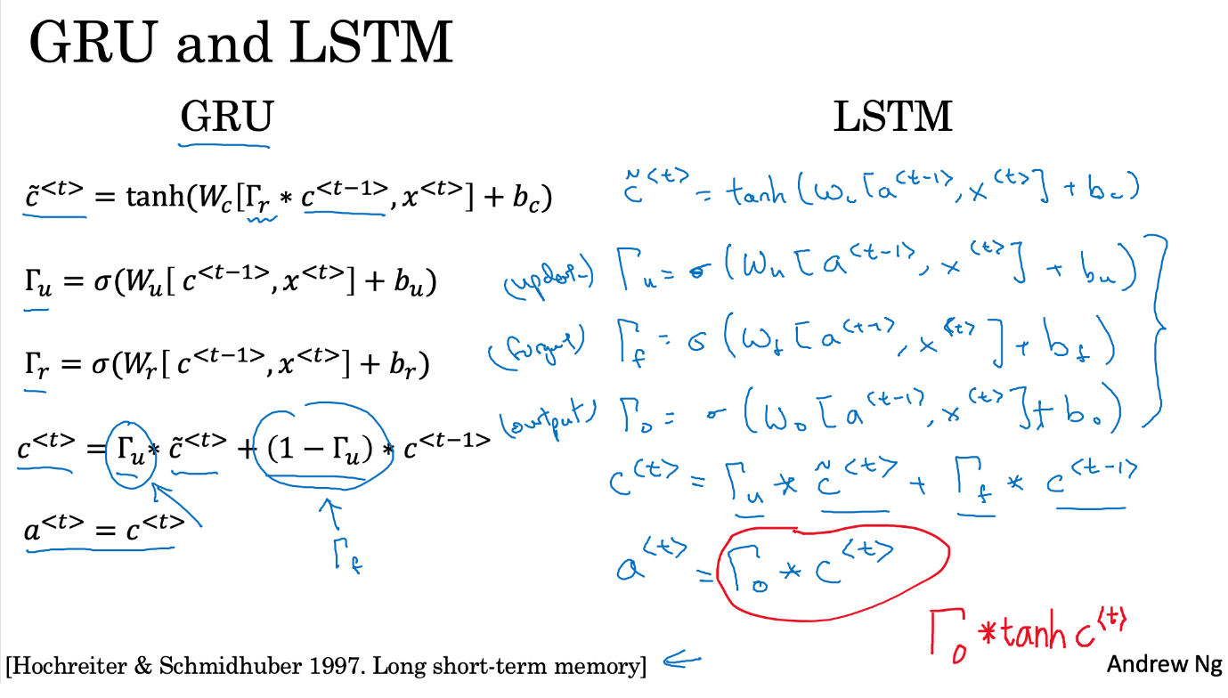
We learned about the GRU, or gated recurrent units, and how that can allow we to learn very long range connections in a sequence. The other type of unit that allows we to do this very well is the LSTM or the long short term memory units, and this is even more powerful than the GRU. Let’s take a look.
Here are the equations from the previous video for the GRU. And for the GRU, we had a^{<t>} = c^{<t>}, and two gates, the optic gate and the relevance gate, \tilde{c}^{<t>}, which is a candidate for replacing the memory cell, and then we use the update gate, \Gamma_u, to decide whether or not to update c^{<t>} using \tilde{c}^{<t>}.
The LSTM is an even slightly more powerful and more general version of the GRU, and is due to Sepp Hochreiter and Jurgen Schmidhuber1, c.f. Hochreiter and Schmidhuber (1997). And this was a really seminal paper, a huge impact on sequence modelling.
1 with many interesting talks online
I think this paper is one of the more difficult to read. It goes quite along into theory of vanishing gradients. And so, I think more people have learned about the details of LSTM through maybe other places than from this particular paper even though I think this paper has had a wonderful impact on the Deep Learning community.
But these are the equations that govern the LSTM. So, we continue to the memory cell, c, and the candidate value for updating it, \tilde{c}^{<t>}, will be this, and so on. Notice that for the LSTM, we will no longer have the case that a^{<t>} =c^{<t>}. So, this is what we use. And so, this is just like the equation on the left except that with now, more specially use a^{<t>} there or a^{<t-1>} instead of c^{<t-1>}. And we’re not using this gamma or this relevance gate. Although we could have a variation of the LSTM where we put that back in, but with the more common version of the LSTM, doesn’t bother with that. And then we will have an update gate, same as before. So, W updates and we’re going to use a^{<t-1>} here, x^{<t>} + b_u. And one new property of the LSTM is, instead of having one update gate control, both of these terms, we’re going to have two separate terms. So instead of gamma_u and one minus gamma_u, we’re going have \Gamma_u here. And forget gate, which we’re going to call \Gamma_f. So, this gate, \Gamma_f, is going to be sigmoid of pretty much what you’d expect, x^{<t>}+ b_f. And then, we’re going to have a new output gate which is \sigma(W_o)+ b_o. And then, the update value to the memory so will be c^{<t>}=\Gamma_u. And this asterisk denotes element-wise multiplication. This is a vector-vector element-wise multiplication, plus, and instead of one minus gamma u, we’re going to have a separate forget gate, \Gamma_f * c^{<t-1>}. So this gives the memory cell the option of keeping the old value c^{t-1} and then just adding to it, this new value, \tilde{c}^{<t>}. So, use a separate update and forget gates. So, this stands for update, forget, and output gate.
And then finally, instead of a^{<t>} = c^{<t>} \quad \text{(GRU)} \qquad a^{<t>} = \Gamma_0 * \tanh( c^{<t>}) \quad \text{(LSTM)} .
So, these are the equations that govern the LSTM and we can tell it has three gates instead of two. So, it’s a bit more complicated and it places the gates into slightly different places. So, here again are the equations governing the behavior of the LSTM.
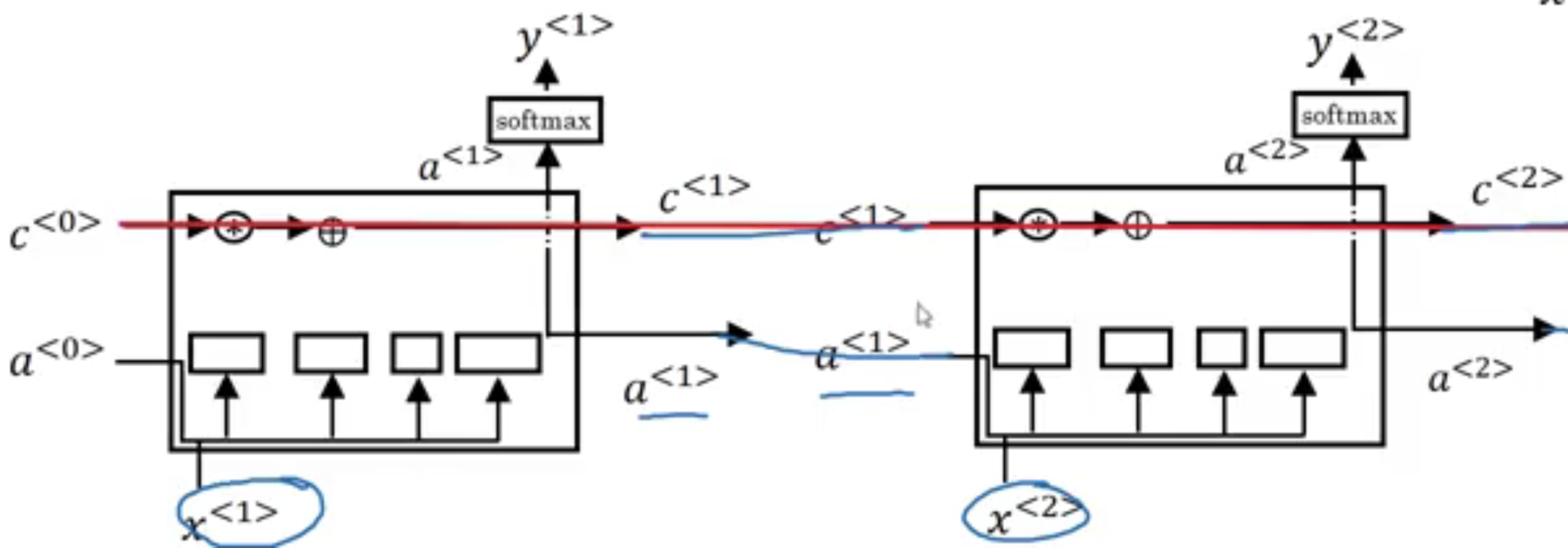
Once again, it’s traditional to explain these things using pictures. So let me draw one here. And if these pictures are too complicated, don’t worry about it. I personally find the equations easier to understand than the picture. But I’ll just show the picture here for the intuitions it conveys. The bigger picture here was very much inspired by a blog post due to Chris Ola, titled Understanding LSTM Network, and the diagram drawing here is quite similar to one that he drew in his blog post. But the key thing is to take away from this picture are maybe that we use a^{<t-1>} and x^{<t>} to compute all the gate values. In this picture, we have a^{<t-1>}, x^{<t>} coming together to compute the forget gate, to compute the update gates, and to compute output gate. And they also go through a tanh to compute \tilde{c}^{<t>}. And then these values are combined in these complicated ways with element-wise multiplies and so on, to get c^{<t>} from the previous c^{<t-1>}. Now, one element of this is interesting as we have a bunch of these in parallel. So, that’s one of them and we connect them. We then connect these temporally. So it does the input x^{<1>} then x^{<2>}, x^{<3>}. So, we can take these units and just hold them up as follows, where the output a at the previous timestep is the input a at the next timestep, the c. I’ve simplified to diagrams a little bit in the bottom. And one cool thing about this you’ll notice is that there’s this line at the top that shows how, so long as we set the forget and the update gate appropriately, it is relatively easy for the LSTM to have some value c_0 and have that be passed all the way to the right to have your, maybe, c^{<3>}=c^{<0>}. And this is why the LSTM, as well as the GRU, is very good at memorizing certain values even for a long time, for certain real values stored in the memory cell even for many, many timesteps.
So, that’s it for the LSTM.
As we can imagine, there are also a few variations on this that people use. Perhaps, the most common one is that instead of just having the gate values be dependent only on a_{t-1}, x^{<t>}, sometimes, people also sneak in there the values c_{t-1} as well. This is called a peephole connection, introduced in Gers and Schmidhuber (2000) Not a great name maybe but you’ll see, peephole connection. What that means is that the gate values may depend not just on a^{<t-1>} and on x^{<t>}, but also on the previous memory cell value, and the peephole connection can go into all three of these gates’ computations. So that’s one common variation we see of LSTMs. One technical detail is that these are, say, 100-dimensional vectors. So if we have a 100-dimensional hidden memory cell unit, and so is this. And the, say, fifth element of c^{t-1} affects only the fifth element of the corresponding gates, so that relationship is one-to-one, where not every element of the 100-dimensional c^{<t-1>} can affect all elements of the case. But instead, the first element of c^{<t-1>} affects the first element of the case, second element affects the second element, and so on. But if we ever read the paper and see someone talk about the peephole connection, that’s when they mean that c^{<t-1>} is used to affect the gate value as well. So, that’s it for the LSTM.
When should we use a GRU? And when should we use an LSTM?
There isn’t widespread consensus in this. And even though I presented GRUs first, in the history of deep learning, LSTMs actually came much earlier, and then GRUs were relatively recent invention that were maybe derived as Pavia’s simplification of the more complicated LSTM model. Researchers have tried both of these models on many different problems, and on different problems, different algorithms will win out. So, there isn’t a universally-superior algorithm which is why I want to show we both of them. But I feel like when I am using these, the advantage of the GRU is that it’s a simpler model and so it is actually easier to build a much bigger network, it only has two gates, so computationally, it runs a bit faster. So, it scales the building somewhat bigger models but the LSTM is more powerful and more effective since it has three gates instead of two. If we want to pick one to use, I think LSTM has been the historically more proven choice. So, if we had to pick one, I think most people today will still use the LSTM as the default first thing to try. Although, I think in the last few years, GRUs had been gaining a lot of momentum and I feel like more and more teams are also using GRUs because they’re a bit simpler but often work just as well. It might be easier to scale them to even bigger problems. So, that’s it for LSTMs. Well, either GRUs or LSTMs, you’ll be able to build neural network that can capture much longer range dependencies.
The correct version of the final equation in the output gate is here:
https://www.coursera.org/learn/nlp-sequence-models/supplement/xdv6z/long-short-term-memory-lstm-correction
Computing Accuracy
To compare the accuracy, just follow the following steps:
- Pass test set through the model
- Get arg max across the prediction array
- Mask padded tokens
- Compare with the true labels.
Reflections on this unit
- What is the vanishing and exploding gradient problem in RNNs?
- How can we measure the ability of RNN to access data from many time steps back?
- What is the nature of the hidden state in RNNs?
- short term memory
- What is the nature of the internal state in RNNs?
- long term memory
- How are gradients updated in the LSTMs?
- what is the constant error carousel in LSTMs?
- how does it solve the vanishing gradient problem?
- How does gating work in LSTMs?
- Are the gates binary?
- what is the idea behind a peekhole LSTM
- what is the idea of the bLSTM
- Are all LSTMs stacked, cam we have a single layer LSTM?
Resources:
Intro to optimization in deep learning: Gradient Descent (Tutorial) Ayoosh Kathuria
Article on Learning Rate Schedules by Hafidz Zulkifli.
Stochastic Weight Averaging (Paper)
The Unreasonable Effectiveness of Recurrent Neural Networks by Andrej Karpathy
References
Citation
@online{bochman2020,
  author = {Bochman, Oren},
  title = {LSTMs and {Named} {Entity} {Recognition}},
  date = {2020-11-16},
  url = {https://orenbochman.github.io/notes-nlp/notes/c3w3/},
  langid = {en}
}