These are my notes for Week 3 notes for the Natural Language Processing with Probabilistic Models Course in the Natural Language Processing Specialization Offered by DeepLearning.AI on Coursera.
- Conditional probabilities
- Text pre-processing
- Language modeling
- Perplexity
- K-smoothing
- N-grams
- Backoff
- Tokenization
TL;DR - Autocomplete and Language Models
This week we learn how to model a language using N-grams. Starting from the definition of conditional probability we develop the probabilities of sequences of words. Next we add start and end of sentences tokens to our word sequence model. Next we add tokens to represent out of vocabulary words. Then we tackle sparsity by implementing smoothing and backoff. Finally we consider how to evaluate our language model.
In the labs we preprocess a corpus to create an N-gram language model. We then build the language model and evaluate it using perplexity.
In the assignment for this week, we build a language model to generate autocomplete a text fragment. We will also evaluate the perplexity of the model.
N-Grams Overview
Recall how Firth suggested a distributional view of semantics?
Previously we used a vector space model to represent this idea. Now we dive deeper and develop a model for distributional semantics using probabilities of sequences of words. Once we can estimate these probabilities we can predict the next word in a sentence.
N-gram refer to howe we model the a sequence of N words. For example, a bigram model would model the probability of a word given the previous word. A trigram model would model the probability of a word given the previous bigram. And so on. These probabilities are derived by counting frequencies in a corpus of texts.
N-grams are fundamental and give we a foundation that will allow we to understand more complicated models in the specialization. They form the theoretical under pinning for the next two courses.
N-grams models allow us to predict the probabilities of certain words happening in a specific sequence. Using that, we can build an auto-correct or even a search suggestion tool.
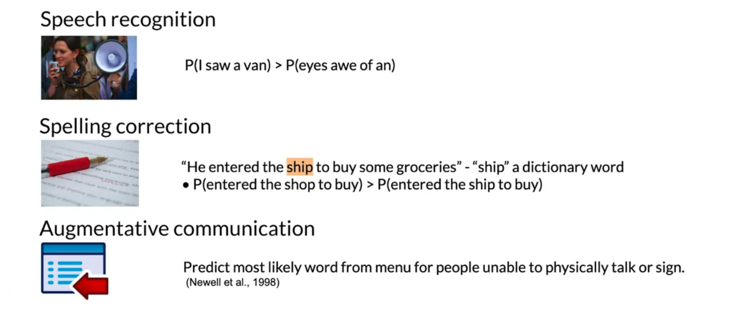
Other applications of N-gram language modeling include:
- Speech recognition
- Spelling correction
- Augmentative communication
This week we are going to learn to:
- Process a text corpus to N-gram language model
- Handle out of vocabulary words
- Implement smoothing for previously unseen N-grams
- Language model evaluation
N-grams and Probabilities
Before we start computing probabilities of certain sequences, we need to first define what is an N-gram language model:
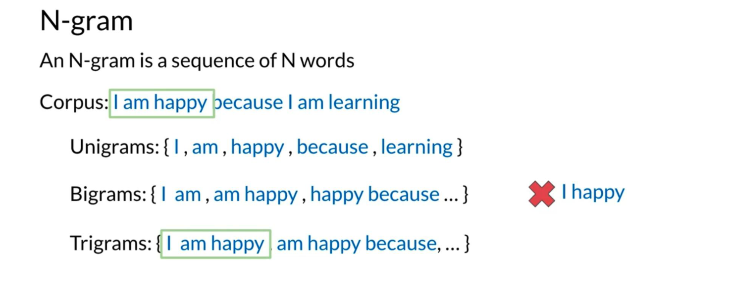
Now given the those definitions, we can label a sentence as follows:

In other notation we can write:
w_1^m = w_1 w_2 w_3 ... w_m w_1^3 = w_1 w_2 w_3 w_{m-2}^m = w_{m-2} w_{m-1} w_m
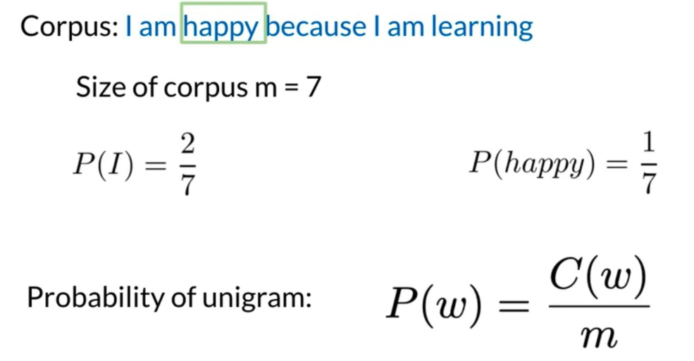
Given the following corpus: I am happy because I am learning.
Size of corpus m = 7.
P(I) = \frac{1}{7}
P(happy) = \frac{1}{7}
To generalize, the probability of a unigram is
P(w) = \frac{C(w)}{m}
Where C(w) is the count of the word in the corpus and m is the size of the corpus.
Bigram Probability:
Trigram Probability:
To compute the probability of a trigram: P(w_3 | w_1^2) = \frac{C(w_1^2 w_3)}{C(w_1^2)}
C(w_1^2 w_3) = C(w_1 w_2 w_3) = C(w_1^3)
N-gram Probability:
P(w_n | w_1^{n-1}) = \frac{C(w_1^{n-1} w_n)}{C(w_1^{n-1})}
C(w_1^{n-1} w_n) = C(w_1^n)
Sequence Probabilities
We just saw how to compute sequence probabilities, their short comings, and finally how to approximate N-gram probabilities. In doing so, we try to approximate the probability of a sentence. For example, what is the probability of the following sentence: The teacher drinks tea. To compute it, we will make use of the following:
P(B|A) = \frac{P(A,B)}{P(A)} \Rightarrow P(A,B) = P(A)P(B|A)
P(A,B,C,D) = P(A)P(B|A)P(C|A,B)P(D|A,B,C)
To compute the probability of a sequence, we can compute the following:
P(\text{The teacher drinks tea}) = P(\text{The})P(\text{teacher}|\text{The})P(\text{drinks}|\text{The teacher})P(\text{tea}|\text{The teacher drinks})
One of the main issues with computing the probabilities above is the corpus rarely contains the exact same phrases as the ones we computed your probabilities on. Hence, we can easily end up getting a probability of 0. The Markov assumption indicates that only the last word matters. Hence:
\text{Bigram} \qquad P(w_n | w_1^{n-1}) \approx P(w_n | w_{n-1})
\text{Trigram} \qquad P(w_n | w_1^{n-1}) \approx P(w_n | w_{n-2}^{n-1})
\text{N-gram} \qquad P(w_n | w_1^{n-1}) \approx P(w_n | w_{n-N+1}^{n-1})
We can model the entire sentence as follows:
P(w_1^n) = P(w_1)P(w_2|w_1)P(w_3|w_2)P(w_4|w_3) ... P(w_n|w_{n-1}) = \prod_{i=1}^{n} P(w_i|w_{i-1})
P(w_1^n) = P(w_1)P(w_2|w_1)P(w_3|w_2)P(w_4|w_3) ... P(w_n|w_{n-1}) = \prod_{i=1}^{n} P(w_i|w_{i-1})
Starting and Ending Sentences
We usually start and end a sentence with the following tokens respectively: <s> </s>.
When computing probabilities using a unigram, we can append an <s> in the beginning of the sentence. To generalize to an N-gram language model, we can add N-1 start tokens <s>.
For the end of sentence token </s>, we only need one even if it is an N-gram. Here is an example:
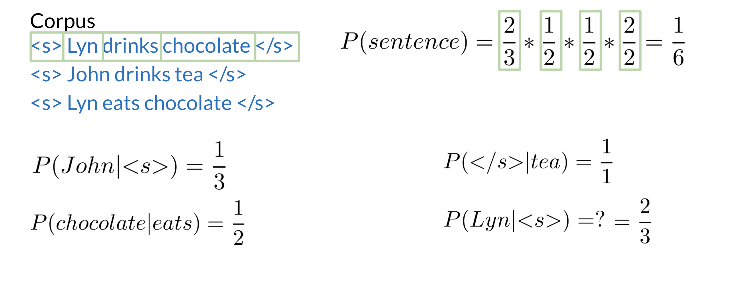
Make sure we know how to compute the probabilities above!
Lecture notebook: Corpus preprocessing for N-grams
The N-gram Language Model
We covered a lot of concepts in the previous video. We have seen:
- Count matrix c.f Figure 7
- Probability matrix c.f Figure 8
- Language model c.f. Figure 9
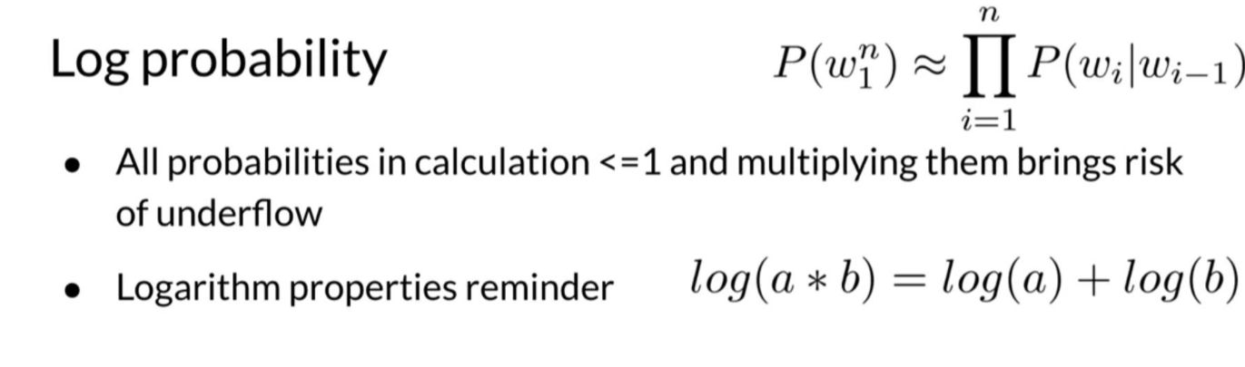
- Log probability c.f Figure 10 to avoid underflow
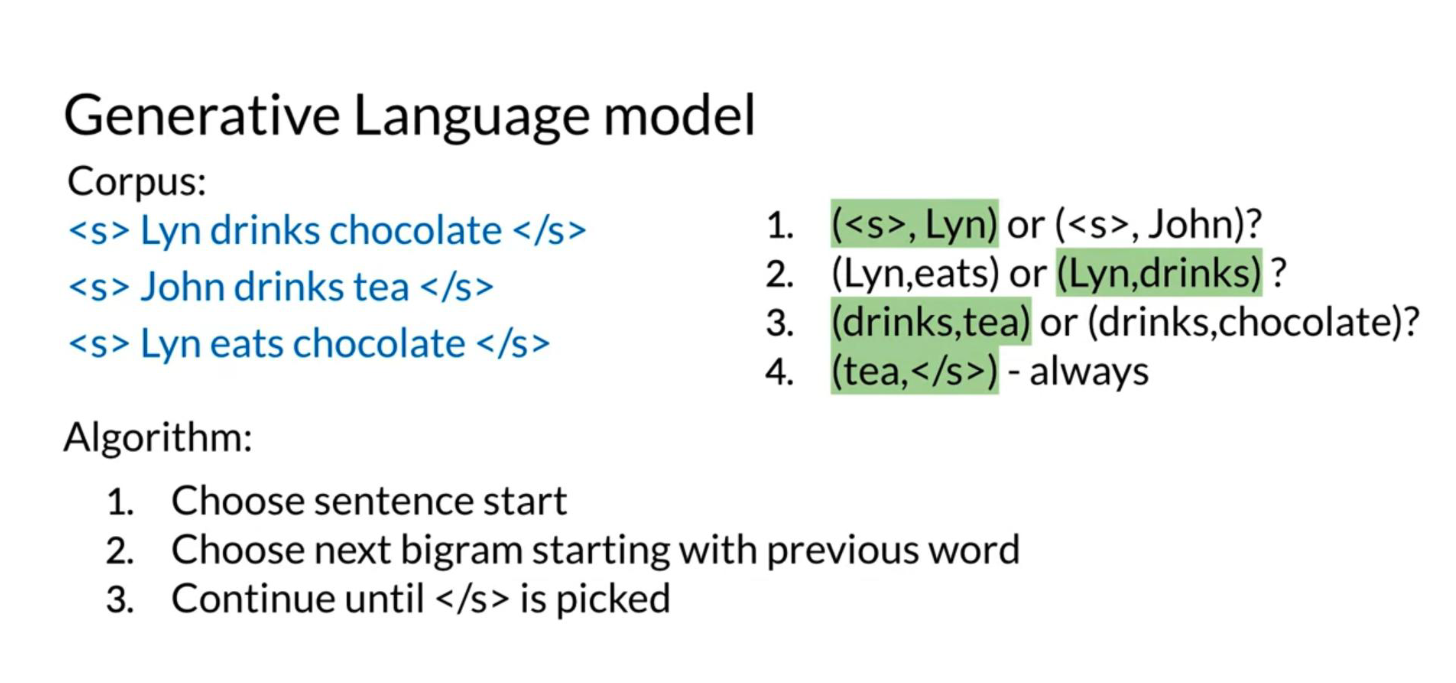
- Generative language model c.f. Figure 11
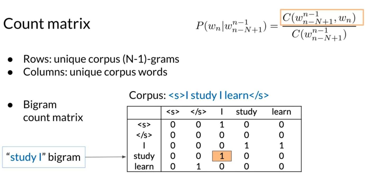
In the count matrix:
- Rows correspond to the unique corpus N-1 grams.
- Columns correspond to the unique corpus words.
Here is an example of the count matrix of a bigram.
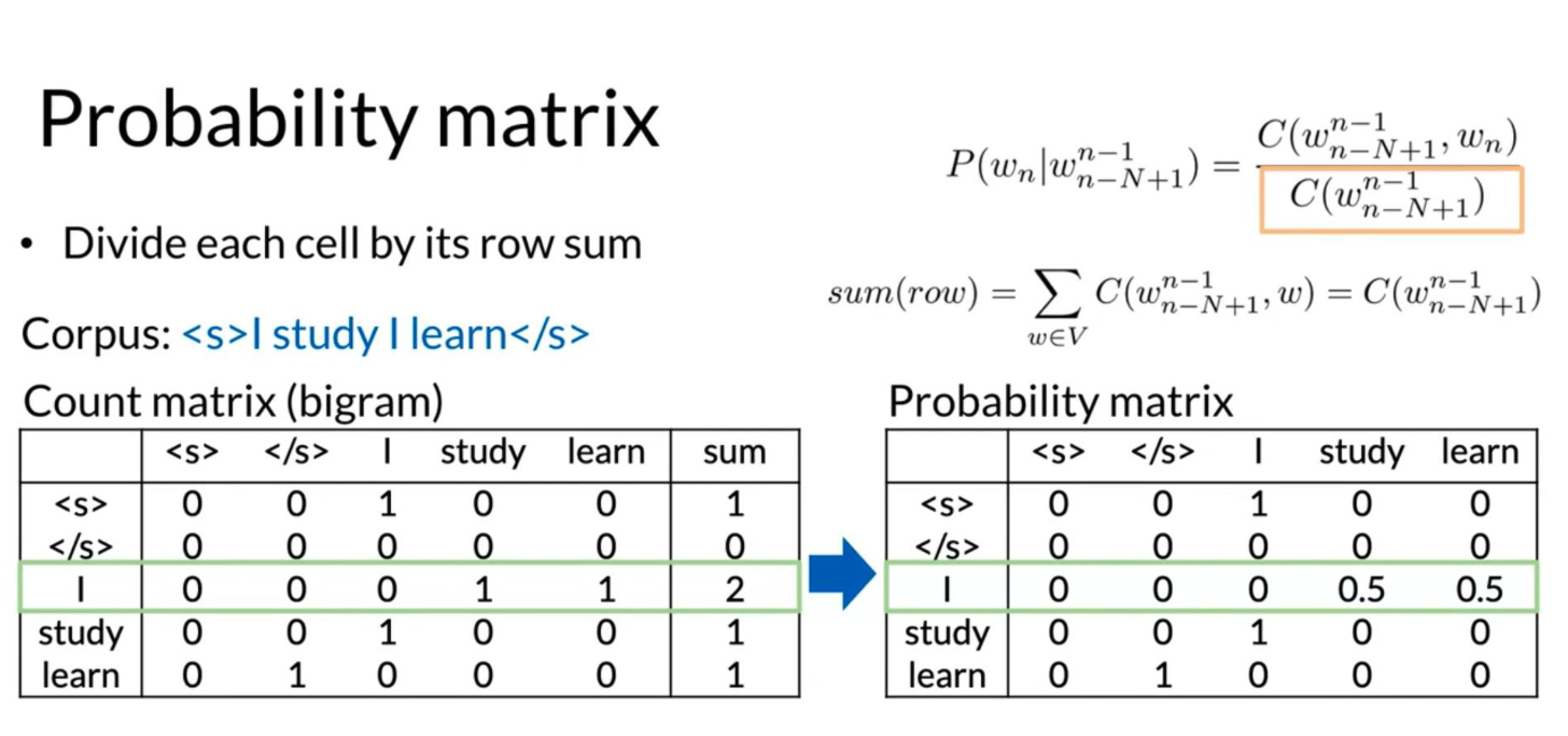
To convert it into a probability matrix, we can use the following formula:
P(w_n \mid w^{n-1}_{n-N+1}) = \frac{C(w^{n-1}_{n-N+1}, w_n)}{C(w^{n-1}_{n-N+1})} \tag{1}
sum(row) = \sum_{w \in V} C(w^{n-1}_{n-N+1}, w) = C(w^{n-1}_{n-N+1}) \tag{2}
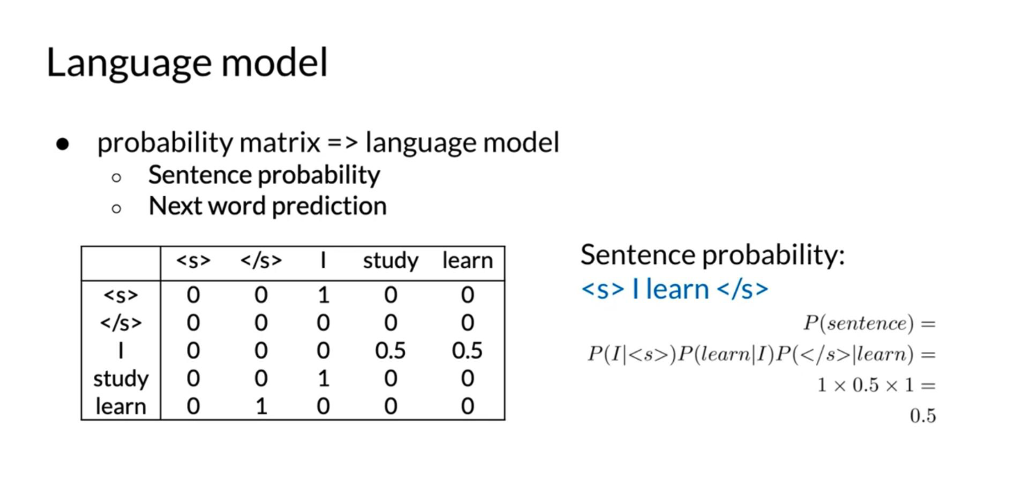
Now given the probability matrix, we can generate the language model. We can compute the sentence probability and the next word prediction.
To compute the probability of a sequence, we needed to compute:
\begin{align*} P(w_1^n) &= P(w_1)P(w_2|w_1)P(w_3|w_2)P(w_4|w_3) \ldots P(w_n|w_{n-1}) \\ &= \prod_{i=1}^{n} P(w_i | w_{i-1}) \end{align*} \tag{3}
To avoid underflow, we can multiply by the log.
\begin{align*} \log P(w_1^n) &= \log P(w_1) + \log P(w_2|w_1) + \log P(w_3|w_2) + \ldots+ \log P(w_n|w_{n-1}) \\ & = \sum_{i=1}^{n} \log P(w_i|w_{i-1}) \end{align*} \tag{4}
Finally, we can create a generative language model.
Lecture notebook: Building the language model
Language Model Evaluation
Splitting the Data We will now discuss the train/val/test splits and perplexity.
| Smaller Corpora: | Larger Corpora: | |
|---|---|---|
| train | 80% | 98% |
| test | 10% | 1% |
| val | 10% | 1% |
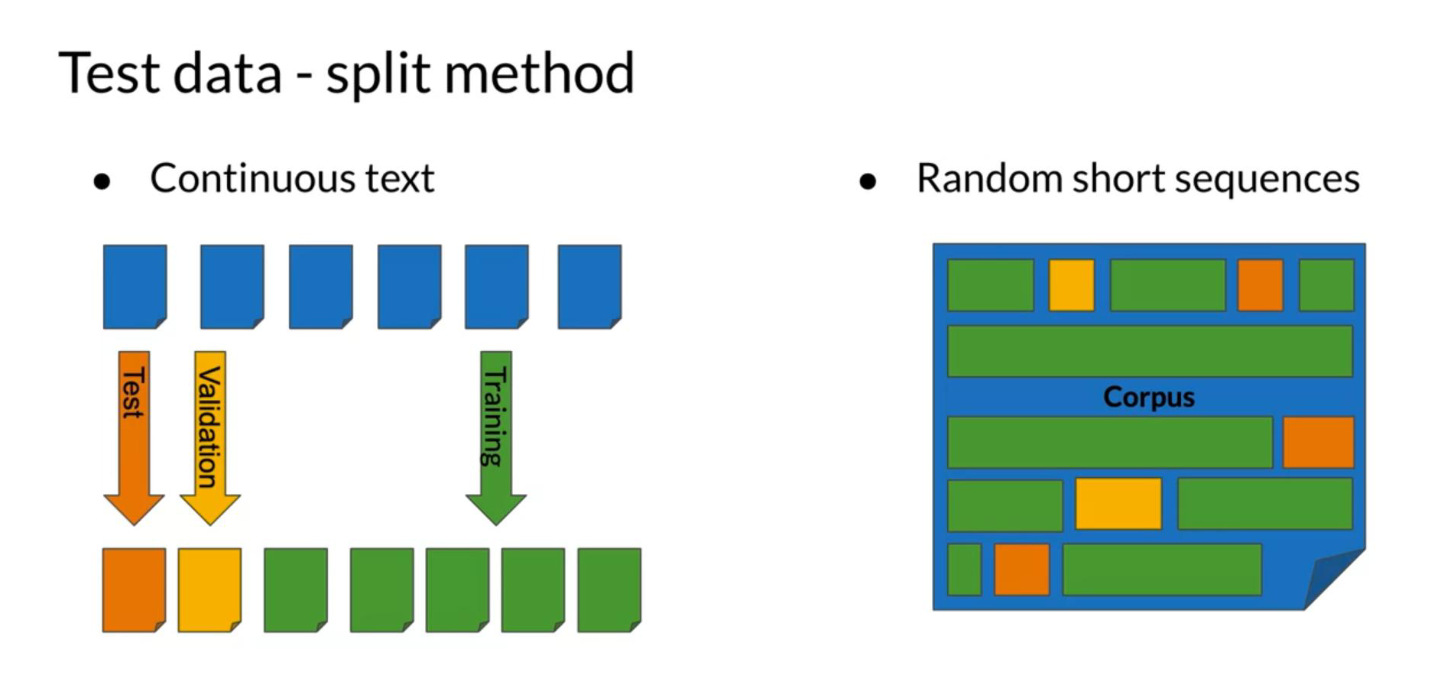
There are two main methods for splitting the data:
Perplexity
Perplexity is used to tell us whether a set of sentences look like they were written by humans rather than by a simple program choosing words at random. A text that is written by humans is more likely to have lower perplexity, where a text generated by random word choice would have a higher perplexity.
Concretely, here are the formulas to calculate perplexity.
PP(W) = P(s_1, s_2, \ldots, s_m)^{-\frac{1}{m}}
PP(W) = \sqrt{ \prod_{i=1}^{m} \prod_{j=1}^{|s_i|} \frac{1}{P(w_j^{(i)} | w_{j-1}^{(i)})}}
w_j^{(i)} corresponds to the jth word in the ith sentence. If we were to concatenate all the sentences then w_i is the ith word in the test set. To compute the log perplexity, we go from:
PP(W) = \sqrt{ \prod_{i=1}^{m} \frac{1}{P(w_i | w_{i-1})}}
To
log PP(W) = -\frac{1}{m} \sum_{i=1}^{m} \log_2 P(w_i | w_{i-1})
Out of Vocabulary Words
Many times, we will be dealing with unknown words in the corpus. So how do we choose your vocabulary? What is a vocabulary?
A vocabulary is a set of unique words supported by your language model. In some tasks like speech recognition or question answering, we will encounter and generate words only from a fixed set of words. Hence, a closed vocabulary.
Open vocabulary means that we may encounter words from outside the vocabulary, like a name of a new city in the training set. Here is one recipe that would allow we to handle unknown words.
- Create vocabulary V
- Replace any word in corpus and not in V by <UNK>
- Count the probabilities with <UNK> as with any other word
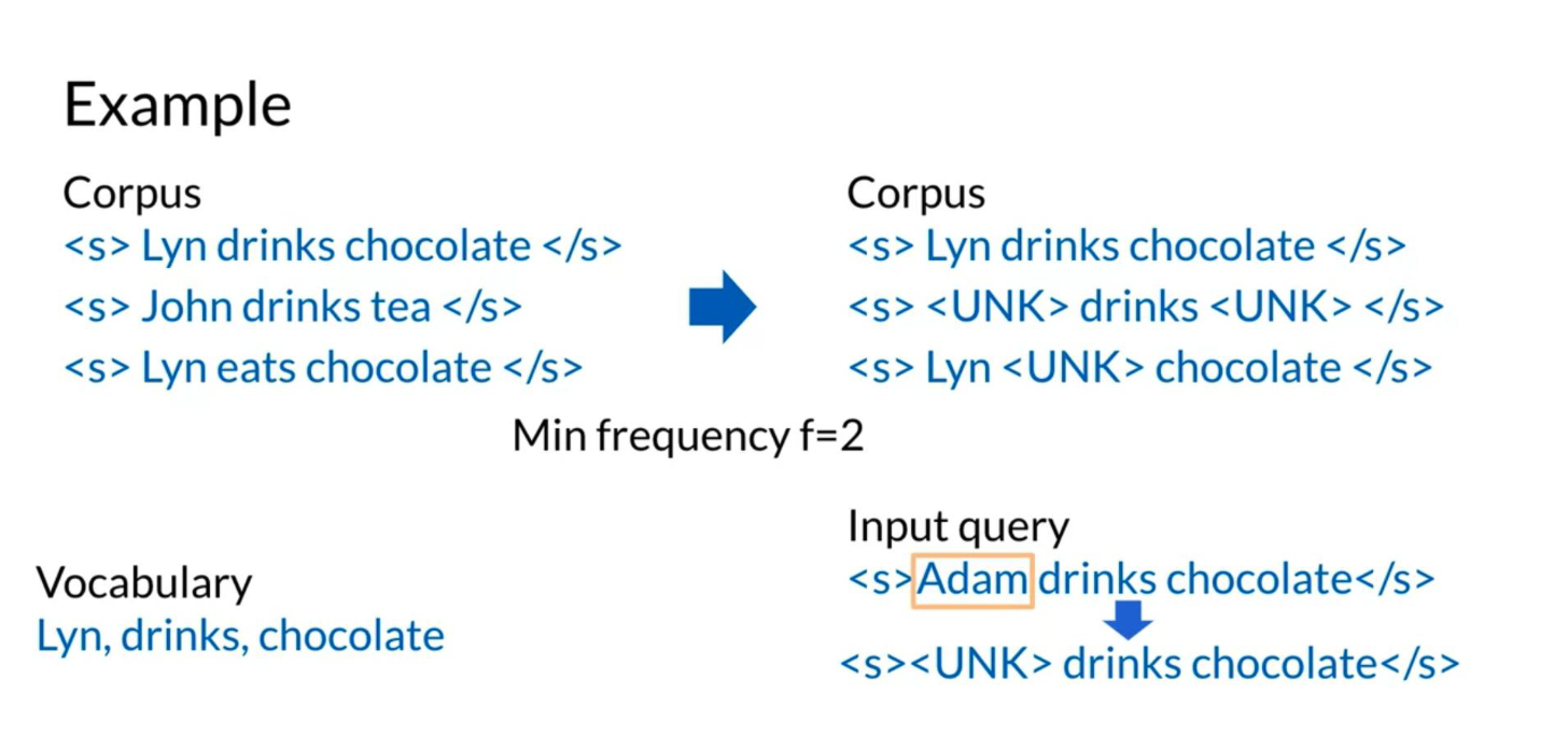
The example above shows how we can use min_frequency and replace all the words that show up fewer times than min_frequency by UNK. We can then treat UNK as a regular word.
Criteria to create the vocabulary
- Min word frequency f
- Max |V|, include words by frequency
- Use <UNK> sparingly (Why?)
- Perplexity - only compare LMs with the same V
Out of Vocabulary Words
Smoothing
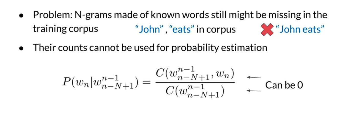
The three main concepts covered here are dealing with missing n-grams, smoothing, and Backoff and interpolation.
P(w_n | w^{n-1}_{n-N+1}) = \frac{C(w^{n-1}_{n-N+1}, w_n)}{C(w^{n-1}_{n-N+1})} \qquad \text{can be 0} \tag{5}
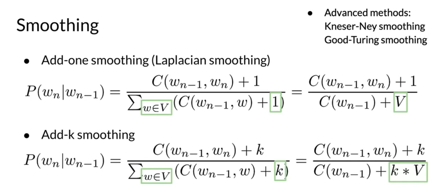
Hence we can add-1 smoothing as follows to fix that problem:
P(w_n | w_{n-1}) = \frac{C(w_{n-1}, w_n) + 1}{\sum_{w \in V} (C(w_{n-1}, w) + 1)} = \frac{C(w_{n-1}, w_n) + 1}{C(w_{n-1}) + V} \qquad \tag{6}
Add-k smoothing is very similar:
P(w_n | w_{n-1}) = \frac{C(w_{n-1}, w_n) + k}{\sum_{w \in V} (C(w_{n-1}, w) + k)} =\frac{C(w_{n-1}, w_n) + k}{C(w_{n-1}) + k\times V} \qquad \tag{7}
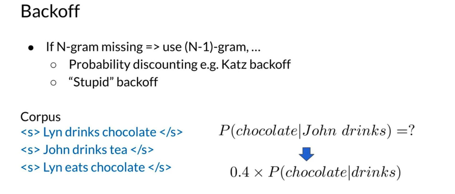
When using back-off:
If N-gram missing => use (N-1)-gram, …: Using the lower level N-grams (i.e. (N-1)-gram, (N-2)-gram, down to unigram) distorts the probability distribution. Especially for smaller corpora, some probability needs to be discounted from higher level N-grams to use it for lower level N-grams.
Probability discounting e.g. Katz backoff: makes use of discounting.
“Stupid” backoff: If the higher order N-gram probability is missing, the lower order N-gram probability is used, just multiplied by a constant. A constant of about 0.4 was experimentally shown to work well.
Here is a visualization of the backoff process.
We can also use interpolation when computing probabilities as follows:
\hat{P}(w_n | w_{n-2} W_{n-1}) = \lambda_1 \times P(w_n | w_{n-2} w_{n-1}) + \lambda_2 \times P(w_n | w_{n-1}) + \lambda_3 \times P(w_n) \qquad \tag{8}
Where
\sum_i \lambda_i = 1
Week Summary
This week we learned the following concepts
- N-Grams and probabilities
- Approximate sentence probability from N-Grams
- Build a language model from a corpus
- Fix missing information
- Out of vocabulary words with <UNK>
- Missing N-Gram in corpus with smoothing, backoff and interpolation
- Evaluate language model with perplexity
- Coding assignment!
Lecture notebook: Language model generalization
Resources:
References
Citation
@online{bochman2020,
  author = {Bochman, Oren},
  title = {Autocomplete and {Language} {Models}},
  date = {2020-10-24},
  url = {https://orenbochman.github.io/notes-nlp/notes/c2w3/},
  langid = {en}
}