Part of Speech Tagging and Hidden Markov Models

course banner

Figure 1

Figure 2

Learning Objectives

• Markov chains
• Hidden Markov models
• Part-of-speech tagging
• Viterbi algorithm
• Transition probabilities
• Emission probabilities

Part of Speech Tagging

Part of Speech Tagging (POS) is the process of assigning a part of speech to a word. By doing so, we will learn the following:

• Markov Chains
• Hidden Markov Models
• Viterbi algorithm

Here is a concrete example:

autocorrect

Figure 3: Learning Objectives

We can use part of speech tagging for:

• Identifying named entities
• Speech recognition
• Coreference Resolution

We can use the probabilities of POS tags happening near one another to come up with the most reasonable output

Lab1: Working with text data

Working with text data

Markov Chains

POS Tagging

Figure 4: POS Tagging

FSM

Figure 5: FSM representation for POS tagging

The circles of the graph represent the states of your model. A state refers to a certain condition of the present moment. We can think of these as the POS tags of the current word.

Q={q_1, q_2, q_3} \qquad \text{ is the set of all states in your model. }

Markov Chains and POS Tags

To help identify the parts of speech for every word, we need to build a transition matrix that gives we the probabilities from one state to another.

FSM

Figure 6: Learning Objectives

In the diagram above, the blue circles correspond to the part of speech tags, and the arrows correspond to the transition probabilities from one part of speech to another. We can populate the table on the right from the diagram on the left. The first row in your A matrix corresponds to the initial distribution among all the states. According to the table, the sentence has a 40% chance to start as a noun, 10% chance to start with a verb, and a 50% chance to start with another part of speech tag.

In more general notation, we can write the transition matrix A, given some states Q, as follows:

FSM

Figure 7: Learning Objectives

Hidden Markov Models

In the previous video, I showed we an example with a simple markov model. The transition probabilities allowed we to identify the transition probability from one POS to another. We will now explore hidden markov models. In hidden markov models we make use of emission probabilities that give we the probability to go from one state (POS tag) to a specific word.

State Transition Graph

Figure 8: Emission probabilities

For example, given that we are in a verb state, we can go to other words with certain probabilities. This emission matrix B, will be used with your transition matrix A, to help we identify the part of speech of a word in a sentence. To populate your matrix B, we can just have a labelled dataset and compute the probabilities of going from a POS to each word in your vocabulary. Here is a recap of what we have seen so far:

HMM

Figure 9: HMM Summary

Note that the sum of each row in your A and B matrix has to be 1. Next, I will show we how we can calculate the probabilities inside these matrices.

Calculating Probabilities

Here is a visual representation on how to calculate the probabilities:

Transition Probabilities

Figure 10: Transition Probabilities

The number of times that blue is followed by purple is 2 out of 3. We will use the same logic to populate our transition and emission matrices. In the transition matrix we will count the number of times tag t_{(i−1)},t{(i)} show up near each other and divide by the total number of times t_{(i−1)} shows up. (which is the same as the number of times it shows up followed by anything else).

Transition Probabilities

Figure 11: Transition Probabilities

1. calculate co-occurrence of tag pairs C(t_{(i-1)},t_{(i)}) \tag{1}

2. calculate the probabilities using the counts P(t_{(i)}|t_{(i-1)}) = \frac{C(t_{(i)}),t_{(i-1)},}{\sum_{i=1}^{N} C(t_{(i-1)})} \tag{2}

Where

C(t_{(i−1)} ,t_{(i)}) is the count of times tag t_{(i-1)} shows up before tag i.

From this we can compute the probability that a tag shows up after another tag.

Populating the Transition Matrix

To populate the transition matrix we have to keep track of the number of times each tag shows up before another tag.

Transition Probabilities

Figure 12: Transition Probabilities

In the table above, we can see that green corresponds to nouns (NN), purple corresponds to verbs (VB), and blue corresponds to other (O). Orange (π) corresponds to the initial state. The numbers inside the matrix correspond to the number of times a part of speech tag shows up right after another one.

To go from O to NN or in other words to calculate P(O∣NN) we have to compute the following:

Transition Probabilities

Figure 13: Transition Probabilities

To generalize:

P(t_{(i)} \mid t_{(i-1)}) = \frac{C(t_{(i)},t_{(i-1)})}{\sum_{j=1}^{N} C(t_{(i-1)},t_{(j)})} \tag{3}

Where:

• C(t_{(i)},t_{(i-1)}) is the count of times tag t_{(i-1)} shows up before tag i.

Unfortunately, sometimes we might not see two POS tags in front each other. This will give we a probability of 0. To solve this issue, we will “smooth” it as follows:

Transition Probabilities

Figure 14: Transition Probabilities

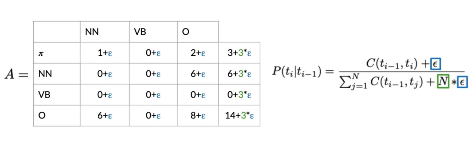
The \epsilon allows we to not have any two sequences showing up with 0 probability. Why is this important?

Populating the Emission Matrix

To populate the emission matrix, we have to keep track of the words associated with their parts of speech tags.

The Emission Matrix

Figure 15: The Emission Matrix

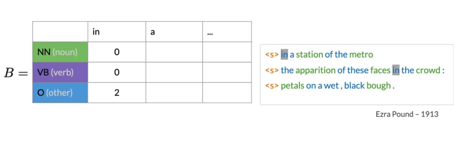
To populate the matrix, we will also use smoothing as we have previously used:

P(w_i \mid t_i) = \frac{C(t_i,w_i)+\epsilon}{\sum_{j=1}^{N} C(t_i,w_j)+ N \times \epsilon} = \frac{C(t_i,w_i)+\epsilon}{\sum_{j=1}^{N} C(t_i)+N\times \epsilon}

Where C(t_i,w_i) is the count associated with how many times the tag t_i is associated with the word w_i. The epsilon above is the smoothing parameter. In the next video, we will talk about the Viterbi algorithm and discuss how we can use the transition and emission matrix to come up with probabilities.

Lab2: Working with text data

Working with text data

The Viterbi Algorithm

The Viterbi algorithm makes use of the transition probabilities and the emission probabilities as follows.

The Emission Matrix

Figure 16: The Viterbi Algorithm

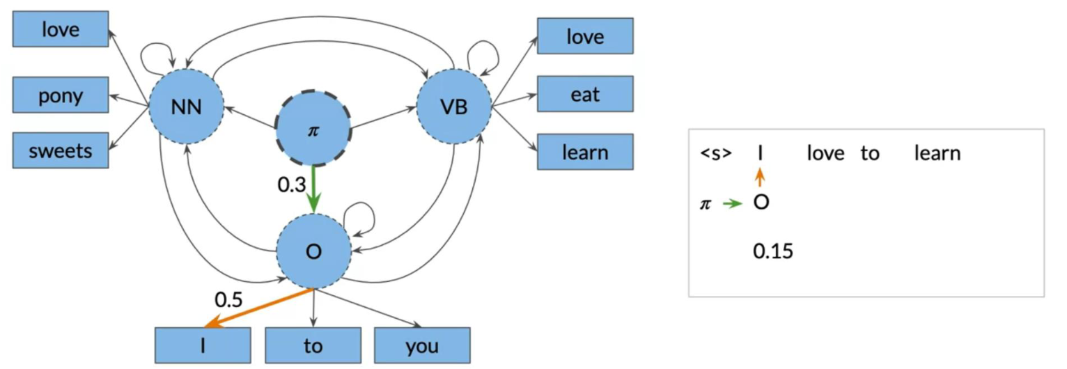
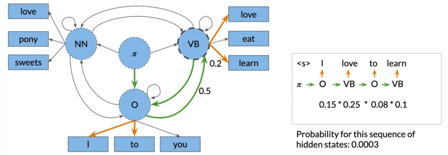
To go from π to O we need to multiply the corresponding transition probability (0.3) and the corresponding emission probability (0.5), which gives we 0.15. We keep doing that for all the words, until we get the probability of an entire sequence.

The Emission Matrix

Figure 17: The Viterbi Algorithm

We can then see how we will just pick the sequence with the highest probability. We will show we a systematic way to accomplish this (Viterbi!).

Viterbi Initialization

We will now populate a matrix C of dimension (num_tags, num_words). This matrix will have the probabilities that will tell we what part of speech each word belongs to.

The Emission Matrix

Figure 18: The Viterbi Initialization

Now to populate the first column, we just multiply the initial π distribution, for each tag, times b_{i,cindex(w_1)}, which is the emission probability of the word 1 given the tag i. Where the i, corresponds to the tag of the initial distribution and the cindex(w_1), is the index of word 1 in the emission matrix. And that’s it, we are done with populating the first column of your new C matrix. We will now need to keep track what part of speech we are coming from. Hence we introduce a matrix D, which allows we to store the labels that represent the different states we are going through when finding the most likely sequence of POS tags for the given sequence of words w_2 ,…,w_k. At first we set the first column to 0, because we are not coming from any POS tag.

The Emission Matrix

Figure 19: The Viterbi Initialization

These two matrices will make more sense in the next videos.

Viterbi: Forward Pass

This will be best illustrated with an example:

Viterbi: Forward Pass

Figure 20: Viterbi: Forward Pass

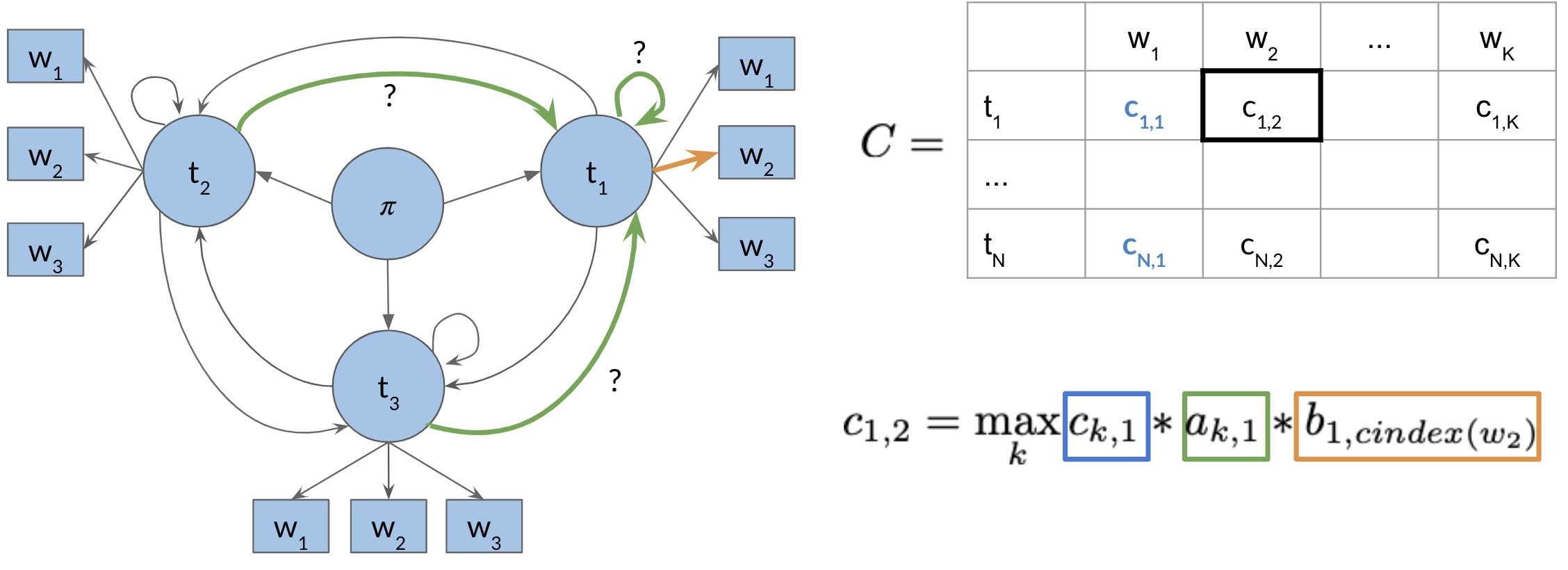
So to populate a cell (i.e. 1,2) in the image above, we have to take the max of [kth cells in the previous column, times the corresponding transition probability of the kth POS to the first POS times the emission probability of the first POS and the current word we are looking at]. We do that for all the cells. Take a paper and a pencil, and make sure we understand how it is done.

The general rule is c_{ij}= max_k c_{k,j-1} \times a_{k,i} \times b_{i,cindex(w_j)}

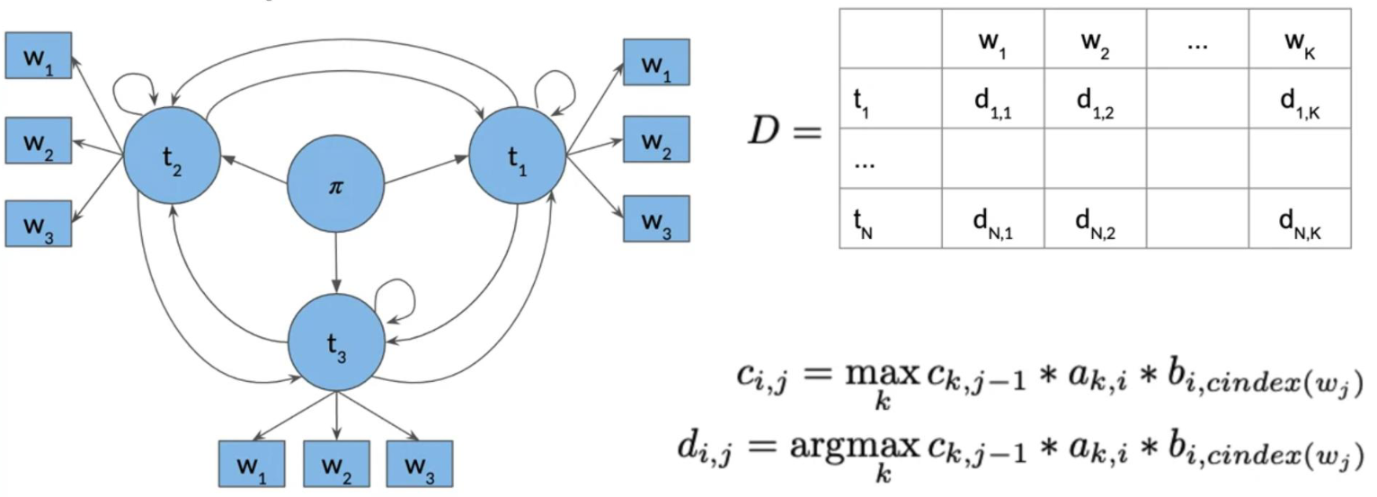
Now to populate the D matrix, we will keep track of the argmax of where we came from as follows:

Note that the only difference between c_{ij} and d_{ij}, is that in the former we compute the probability and in the latter we keep track of the index of the row where that probability came from. So we keep track of which k was used to get that max probability.

Viterbi: Backward Pass

Great, now that we know how to compute A, B, C, and D, we will put it all together and show we how to construct the path that will give we the part of speech tags for your sentence.

Viterbi: Forward Pass

Figure 21: Viterbi: Forward Pass

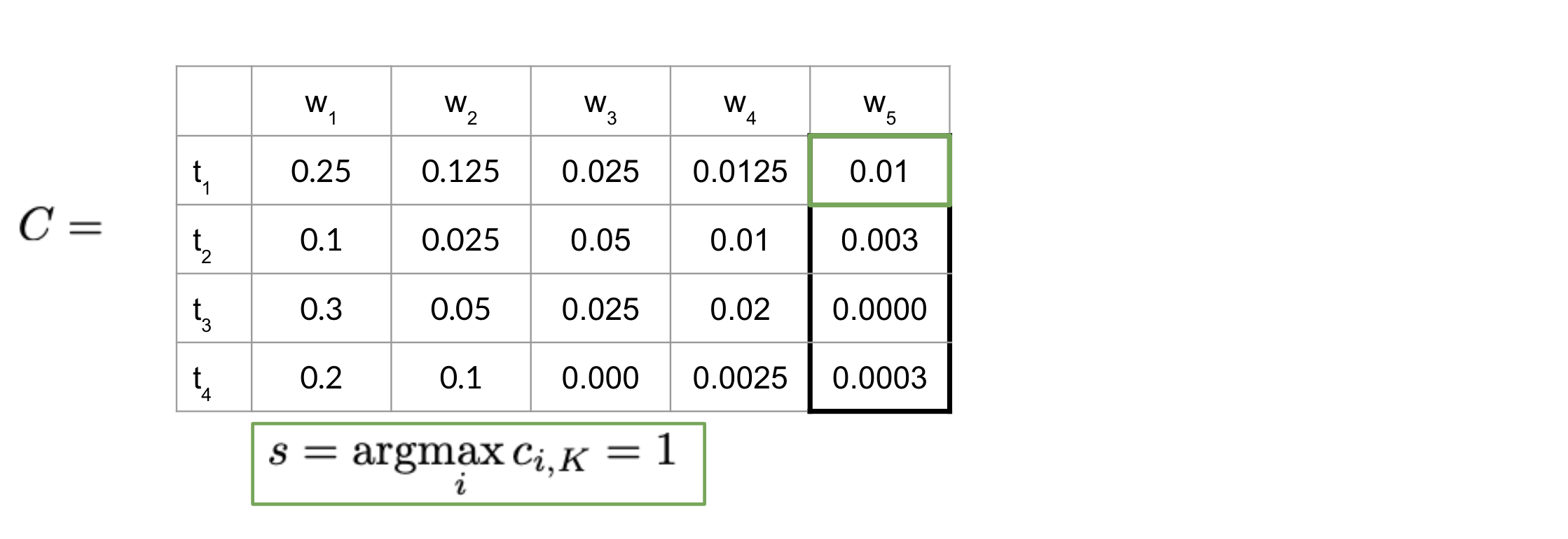
The equation above just gives we the index of the highest row in the last column of C. Once we have that, we can go ahead and start using your D matrix as follows:

Viterbi: Forward Pass

Figure 22: Viterbi: Forward Pass

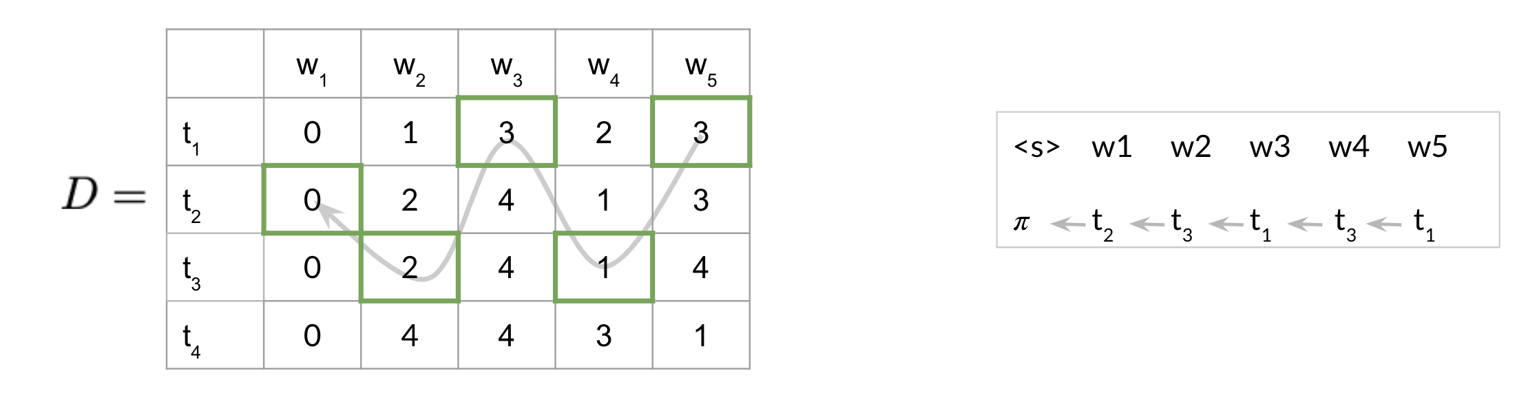
Note that since we started at index one, hence the last word (w5) is t_1. Then we go to the first row of D and what ever that number is, it indicated the row of the next part of speech tag. Then next part of speech tag indicates the row of the next and so forth. This allows we to reconstruct the POS tags for your sentence.

We will be implementing this in this week’s programming assignment.

Assignment

Part-of-speech (POS) tagging