This ungraded lab will explore Reversible Residual Networks. You will use these networks in this week’s assignment that utilizes the Reformer model. It is based on on the Transformer model you already know, but with two unique features. * Locality Sensitive Hashing (LSH) Attention to reduce the compute cost of the dot product attention and * Reversible Residual Networks (RevNets) organization to reduce the storage requirements when doing backpropagation in training.
In this ungraded lab we’ll start with a quick review of Residual Networks and their implementation in Trax. Then we will discuss the Revnet architecture and its use in Reformer.
import traxfrom trax import layers as tl # core building blockimport numpy as np # regular ol' numpyfrom trax.models.reformer.reformer import ( ReversibleHalfResidualV2 as ReversibleHalfResidual,) # unique spotfrom trax import fastmath # uses jax, offers numpy on steroidsfrom trax import shapes # data signatures: dimensionality and typefrom trax.fastmath import numpy as jnp # For use in defining new layer types.from trax.shapes import ShapeDtypefrom trax.shapes import signature
2025-02-10 16:54:01.601593: E external/local_xla/xla/stream_executor/cuda/cuda_fft.cc:477] Unable to register cuFFT factory: Attempting to register factory for plugin cuFFT when one has already been registered
WARNING: All log messages before absl::InitializeLog() is called are written to STDERR
E0000 00:00:1739199241.613582  121997 cuda_dnn.cc:8310] Unable to register cuDNN factory: Attempting to register factory for plugin cuDNN when one has already been registered
E0000 00:00:1739199241.617462  121997 cuda_blas.cc:1418] Unable to register cuBLAS factory: Attempting to register factory for plugin cuBLAS when one has already been registered
---------------------------------------------------------------------------ImportError Traceback (most recent call last)
Cell In[1], line 4 2fromtraximport layers as tl # core building block 3importnumpyasnp# regular ol' numpy----> 4fromtrax.models.reformer.reformerimport (
5 ReversibleHalfResidualV2 as ReversibleHalfResidual,
6 ) # unique spot 7fromtraximport fastmath # uses jax, offers numpy on steroids 8fromtraximport shapes # data signatures: dimensionality and typeImportError: cannot import name 'ReversibleHalfResidualV2' from 'trax.models.reformer.reformer' (/home/oren/work/notes/notes-nlp/.venv/lib/python3.10/site-packages/trax/models/reformer/reformer.py)
Part 1.0 Residual Networks
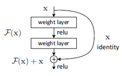
Deep Residual Networks (Resnets) were introduced to improve convergence in deep networks. Residual Networks introduce a shortcut connection around one or more layers in a deep network as shown in the diagram below from the original paper.
Figure 1: Residual Network diagram from original paper
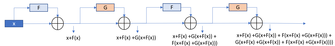
The Trax documentation describes an implementation of Resnets using branch. We’ll explore that here by implementing a simple resnet built from simple function based layers. Specifically, we’ll build a 4 layer network based on two functions, ‘F’ and ‘G’.
Figure 2: 4 stage Residual network
Don’t worry about the lengthy equations. Those are simply there to be referenced later in the notebook.
Part 1.1 Branch
Trax branch figures prominently in the residual network layer so we will first examine it. You can see from the figure above that we will need a function that will copy an input and send it down multiple paths. This is accomplished with a branch layer, one of the Trax ‘combinators’. Branch is a combinator that applies a list of layers in parallel to copies of inputs. Lets try it out! First we will need some layers to play with. Let’s build some from functions.
# simple function taking one input and one outputbl_add1 = tl.Fn("add1", lambda x0: (x0 +1), n_out=1)bl_add2 = tl.Fn("add2", lambda x0: (x0 +2), n_out=1)bl_add3 = tl.Fn("add3", lambda x0: (x0 +3), n_out=1)# try them outx = np.array([1])print(bl_add1(x), bl_add2(x), bl_add3(x))# some information about our new layersprint("name:", bl_add1.name,"number of inputs:", bl_add1.n_in,"number of outputs:", bl_add1.n_out,)
[2] [3] [4]
name: add1 number of inputs: 1 number of outputs: 1
Trax uses the concept of a ‘stack’ to transfer data between layers. For Branch, for each of its layer arguments, it copies the n_in inputs from the stack and provides them to the layer, tracking the max_n_in, or the largest n_in required. It then pops the max_n_in elements from the stack.
Figure 3: One in, one out Branch
On output, each layer, in succession pushes its results onto the stack. Note that the push/pull operations impact the top of the stack. Elements that are not part of the operation (n, and m in the diagram) remain intact.
# n_in = 1, Each bl_addx pushes n_out = 1 elements onto the stackbl_3add1s(x)
(array([2]), array([3]), array([4]))
# n = np.array([10]); m = np.array([20]) # n, m will remain on the stackn ="n"m ="m"# n, m will remain on the stackbl_3add1s([x, n, m])
(array([2]), array([3]), array([4]), 'n', 'm')
Each layer in the input list copies as many inputs from the stack as it needs, and their outputs are successively combined on stack. Put another way, each element of the branch can have differing numbers of inputs and outputs. Let’s try a more complex example.
bl_addab = tl.Fn("addab", lambda x0, x1: (x0 + x1), n_out=1) # Trax figures out how many inputs there arebl_rep3x = tl.Fn("add2x", lambda x0: (x0, x0, x0), n_out=3) # but you have to tell it how many outputs there arebl_3ops = tl.Branch(bl_add1, bl_addab, bl_rep3x)
In this case, the number if inputs being copied from the stack varies with the layer
Figure 4: variable in, variable out Branch
The stack when the operation is finished is 5 entries reflecting the total from each layer.
# Before Running this cell, what is the output you are expecting?y = np.array([3])bl_3ops([x, y, n, m])
Branch has a special feature to support Residual Network. If an argument is ‘None’, it will pull the top of stack and push it (at its location in the sequence) onto the output stack
Figure 5: Branch for Residual
bl_2ops = tl.Branch(bl_add1, None)bl_2ops([x, n, m])
(array([2]), array([1]), 'n', 'm')
### Part 1.2 Residual Model OK, your turn. Write a function ‘MyResidual’, that uses tl.Branch and tl.Add to build a residual layer. If you are curious about the Trax implementation, you can see the code here.
def MyResidual(layer):return tl.Serial(### START CODE HERE ### tl.Branch(layer, None), tl.Add(),### END CODE HERE ### )
# Lets Try itmr = MyResidual(bl_add1)x = np.array([1])mr([x, n, m])
(array([3]), 'n', 'm')
Expected Result (array([3]), ‘n’, ‘m’)
Great! Now, let’s build the 4 layer residual Network in Figure 2. You can use MyResidual, or if you prefer, the tl.Residual in Trax, or a combination!
resfg = tl.Serial(### START CODE HERE #### None, #Fl # x + F(x)# None, #Gl # x + F(x) + G(x + F(x)) etc# None, #Fl# None, #Gl### END CODE HERE ###)
# Lets try itresfg([x1, n, m])
[array([1]), 'n', 'm']
Expected Results (array([1089]), ‘n’, ‘m’)
## Part 2.0 Reversible Residual Networks The Reformer utilized RevNets to reduce the storage requirements for performing backpropagation.
Figure 6: Reversible Residual Networks
The standard approach on the left above requires one to store the outputs of each stage for use during backprop. By using the organization to the right, one need only store the outputs of the last stage, y1, y2 in the diagram. Using those values and running the algorithm in reverse, one can reproduce the values required for backprop. This trades additional computation for memory space which is at a premium with the current generation of GPU’s/TPU’s.
One thing to note is that the forward functions produced by two networks are similar, but they are not equivalent. Note for example the asymmetry in the output equations after two stages of operation.
Figure 7: ‘Normal’ Residual network (Top) vs REversible Residual Network
Part 2.1 Trax Reversible Layers
Let’s take a look at how this is used in the Reformer.
refm = trax.models.reformer.ReformerLM( vocab_size=33000, n_layers=2, mode="train"# Add more options.)refm
Eliminating some of the detail, we can see the structure of the network.
Figure 8: Key Structure of Reformer Reversible Network Layers in Trax
We’ll review the Trax layers used to implement the Reversible section of the Reformer. First we can note that not all of the reformer is reversible. Only the section in the ReversibleSerial layer is reversible. In a large Reformer model, that section is repeated many times making up the majority of the model.
Figure 9: Functional Diagram of Trax elements in Reformer
The implementation starts by duplicating the input to allow the two paths that are part of the reversible residual organization with Dup. Note that this is accomplished by copying the top of stack and pushing two copies of it onto the stack. This then feeds into the ReversibleHalfResidual layer which we’ll review in more detail below. This is followed by ReversibleSwap. As the name implies, this performs a swap, in this case, the two topmost entries in the stack. This pattern is repeated until we reach the end of the ReversibleSerial section. At that point, the topmost 2 entries of the stack represent the two paths through the network. These are concatenated and pushed onto the stack. The result is an entry that is twice the size of the non-reversible version.
Let’s look more closely at the ReversibleHalfResidual. This layer is responsible for executing the layer or layers provided as arguments and adding the output of those layers, the ‘residual’, to the top of the stack. Below is the ‘forward’ routine which implements this.
Figure 10: ReversibleHalfResidual code and diagram
Unlike the previous residual function, the value that is added is from the second path rather than the input to the set of sublayers in this layer. Note that the Layers called by the ReversibleHalfResidual forward function are not modified to support reverse functionality. This layer provides them a ‘normal’ view of the stack and takes care of reverse operation.
Let’s try out some of these layers! We’ll start with the ones that just operate on the stack, Dup() and Swap().
x1 = np.array([1])x2 = np.array([5])# Dup() duplicates the Top of Stack and returns the stackdl = tl.Dup()dl(x1)
(array([1]), array([1]))
# ReversibleSwap() duplicates the Top of Stack and returns the stacksl = tl.ReversibleSwap()sl([x1, x2])
(array([5]), array([1]))
You are no doubt wondering “How is ReversibleSwap different from Swap?”. Good question! Lets look:
Figure 11: Two versions of Swap()
The ReverseXYZ functions include a “reverse” compliment to their “forward” function that provides the functionality to run in reverse when doing backpropagation. It can also be run in reverse by simply calling ‘reverse’.
Just a note about ReversibleHalfResidual. As this is written, it resides in the Reformer model and is a layer. It is invoked a bit differently that other layers. Rather than tl.XYZ, it is just ReversibleHalfResidual(layers..) as shown below. This may change in the future.
---------------------------------------------------------------------------NameError Traceback (most recent call last)
Cell In[19], line 1----> 1 half_res_F =ReversibleHalfResidual(Fl)
2print(type(half_res_F), "\n", half_res_F)
NameError: name 'ReversibleHalfResidual' is not defined
half_res_F([x1, x1]) # this is going to produce an error - why?
---------------------------------------------------------------------------NameError Traceback (most recent call last)
Cell In[20], line 1----> 1half_res_F([x1, x1]) # this is going to produce an error - why?NameError: name 'half_res_F' is not defined
# we have to initialize the ReversibleHalfResidual layer to let it know what the input is going to look likehalf_res_F.init(shapes.signature([x1, x1]))half_res_F([x1, x1])
---------------------------------------------------------------------------NameError Traceback (most recent call last)
Cell In[21], line 2 1# we have to initialize the ReversibleHalfResidual layer to let it know what the input is going to look like----> 2half_res_F.init(shapes.signature([x1, x1]))
3 half_res_F([x1, x1])
NameError: name 'half_res_F' is not defined
Notice the output: (DeviceArray([3], dtype=int32), array([1])). The first value, (DeviceArray([3], dtype=int32) is the output of the “Fl” layer and has been converted to a ‘Jax’ DeviceArray. The second array([1]) is just passed through (recall the diagram of ReversibleHalfResidual above).
The final layer we need is the ReversibleSerial Layer. This is the reversible equivalent of the Serial layer and is used in the same manner to build a sequence of layers.
### Part 2.2 Build a reversible model We now have all the layers we need to build the model shown below. Let’s build it in two parts. First we’ll build ‘blk’ and then a list of blk’s. And then ‘mod’.
Figure 12: Reversible Model we will build using Trax components
blk = [ # a list of the 4 layers shown above### START CODE HERE ###None,None,None,None,]blks = [None, None]### END CODE HERE ###
mod = tl.Serial(### START CODE HERE ###None,None,None,### END CODE HERE ###)mod
/home/oren/work/notes/notes-nlp/.venv/lib/python3.10/site-packages/trax/layers/combinators.py:437: SyntaxWarning: "is not" with a literal. Did you mean "!="?
  if self._mode == 'predict' and self._state[1] is not ():  # pylint: disable=literal-comparison
/home/oren/work/notes/notes-nlp/.venv/lib/python3.10/site-packages/trax/layers/combinators.py:910: SyntaxWarning: "is" with a literal. Did you mean "=="?
  if state[0] is ():  # pylint: disable=literal-comparison
---------------------------------------------------------------------------ValueError Traceback (most recent call last)
Cell In[23], line 1----> 1 mod =tl.Serial( 2### START CODE HERE ### 3None, 4None, 5None, 6### END CODE HERE ### 7) 8 mod
File ~/work/notes/notes-nlp/.venv/lib/python3.10/site-packages/trax/layers/combinators.py:59, in Serial.__init__(self, name, sublayers_to_print, *sublayers) 55def__init__(self, *sublayers, name=None, sublayers_to_print=None):
56super().__init__(
57 name=name, sublayers_to_print=sublayers_to_print)
---> 59 sublayers =_ensure_flat(sublayers) 60self._sublayers = sublayers
61self._n_layers =len(sublayers)
File ~/work/notes/notes-nlp/.venv/lib/python3.10/site-packages/trax/layers/combinators.py:1110, in _ensure_flat(layers) 1108for obj in layers:
1109ifnotisinstance(obj, base.Layer):
-> 1110raiseValueError(
1111f'Found nonlayer object ({obj}) in layers: {layers}')
1112return layers
ValueError: Found nonlayer object (None) in layers: [None, None, None]
Expected Output
Serial[
  Dup_out2
  ReversibleSerial_in2_out2[
    ReversibleHalfResidualV2_in2_out2[
      Serial[
        F
      ]
    ]
    ReversibleSwap_in2_out2
    ReversibleHalfResidualV2_in2_out2[
      Serial[
        G
      ]
    ]
    ReversibleSwap_in2_out2
    ReversibleHalfResidualV2_in2_out2[
      Serial[
        F
      ]
    ]
    ReversibleSwap_in2_out2
    ReversibleHalfResidualV2_in2_out2[
      Serial[
        G
      ]
    ]
    ReversibleSwap_in2_out2
  ]
  Concatenate_in2
]
mod.init(shapes.signature(x1))out = mod(x1)out
---------------------------------------------------------------------------NameError Traceback (most recent call last)
Cell In[24], line 1----> 1mod.init(shapes.signature(x1))
2 out = mod(x1)
3 out
NameError: name 'mod' is not defined
Expected Result DeviceArray([ 65, 681], dtype=int32)
OK, now you have had a chance to try all the ‘Reversible’ functions in Trax. On to the Assignment!
Citation
BibTeX citation:
@online{bochman2021,
  author = {Bochman, Oren},
  title = {Putting the “{Re}” in {Reformer:} {Ungraded} {Lab}},
  date = {2021-04-29},
  url = {https://orenbochman.github.io/notes-nlp/notes/c4w4/lab02.html},
  langid = {en}
}