ARIMA Models
A time series process is a zero-mean autoregressive moving average process if it is given by
y_t = \sum_{i=1}^{p} \phi_i y_{t-i} + \sum_{j=1}^{q} \theta_j \varepsilon_{t-j} + \varepsilon_t,
with \varepsilon_t \sim N(0, v).
When q = 0, we have an AR(p) process.
When p = 0, we have a moving average process of order q or MA(q).
An ARMA process is stable if the roots of the AR characteristic polynomial
stable
\Phi(u) = 1 - \phi_1 u - \phi_2 u^2 - \ldots - \phi_p u^p
lie outside the unit circle, i.e., for all u such that \Phi(u) = 0, |u| > 1.
Equivalently, this happens when the reciprocal roots of the AR polynomial have moduli smaller than 1.
This condition implies stationarity.
An ARMA process is invertible if the roots of the MA characteristic polynomial given by
invertible
\Theta(u) = 1 + \theta_1 u + \dots + \theta_q u^q,
lie outside the unit circle.
Note that \Phi(B) y_t = \Theta(B) \varepsilon_t.
When an ARMA process is stable, it can be written as an infinite order moving average process.
When an ARMA process is invertible, it can be written as an infinite order autoregressive process.
An autoregressive integrated moving average process with orders p, d, and q is a process that can be written as
(1 - B)^d y_t = \sum_{i=1}^{p} \phi_i y_{t-i} + \sum_{j=1}^{q} \theta_j \varepsilon_{t-j} + \varepsilon_t,
in other words, y_t follows an ARIMA(p, d, q) if the d difference of y_t follows an ARMA(p, q).
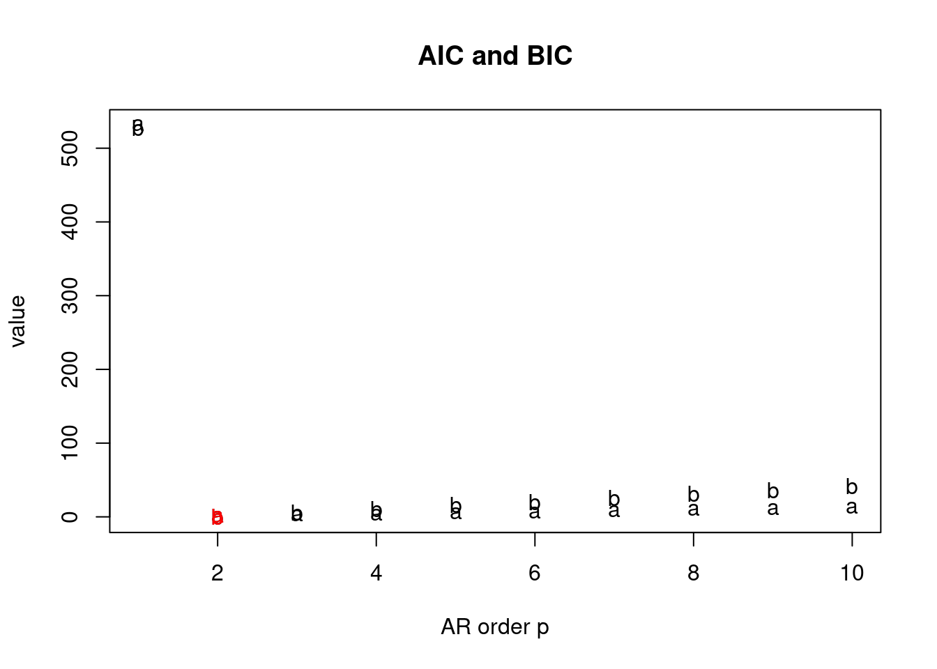
Estimation in ARIMA processes can be done via least squares, maximum likelihood, and also in a Bayesian way. We will not discuss Bayesian estimation of ARIMA processes in this course.
Spectral Density of ARMA Processes
For a given AR(p) process with AR coefficients \phi_1, \dots, \phi_p and variance v, we can obtain its spectral density as
f(\omega) = \frac{v}{2\pi |\Phi(e^{-i\omega})|^2} = \frac{v}{2\pi |1 - \phi_1 e^{-i\omega} - \dots - \phi_p e^{-ip\omega}|^2},
with \omega a frequency in (0, \pi).
The spectral density provides a frequency-domain representation of the process that is appealing because of its interpretability.
For instance, an AR(2) process that has one pair of complex-valued reciprocal roots with modulus 0.7 and a period of \lambda = 12, will show a mode in the spectral density located at a frequency of 2\pi/12. If we keep the period of the process at the same value of 12 but increase its modulus to 0.95, the spectral density will continue to show a mode at 2\pi/12, but the value of f(2\pi/12) will be higher, indicating a more persistent quasi-periodic behavior.
Similarly, we can obtain the spectral density of an ARMA process with AR characteristic polynomial \Phi(u) = 1 - \phi_1 u - \ldots - \phi_p u^p and MA characteristic polynomial \Theta(u) = 1 + \theta_1 u + \ldots + \theta_q u^q, and variance v as
f(\omega) = \frac{v}{2\pi} \frac{|\Theta(e^{-i\omega})|^2}{|\Phi(e^{-i\omega})|^2}.
Note that if we have posterior estimates or posterior samples of the AR/ARMA coefficients and the variance v, we can obtain samples from the spectral density of AR/ARMA processes using the equations above.