The chapter is divided into the following sections:
- Survival and Censoring Times
- A Closer Look at Censoring
- The Kaplan–Meier Survival Curve
- The Log-Rank Test
- Regression Models With a Survival Response
- 11.5.1 The Hazard Function
- 11.5.2 Proportional Hazards
- 11.5.3 Example: Brain Cancer Data
- 11.5.4 Example: Publication Data
- Shrinkage for the Cox Model
- Additional Topics
- 11.7.1 Area Under the Curve for Survival Analysis
- 11.7.2 Choice of Time Scale
- 11.7.3 Time-Dependent Covariates
- 11.7.4 Checking the Proportional Hazards Assumption
- 11.7.5 Survival Trees
- Lab: Survival Analysis
- Exercises

Survival Analysis
There are a number of big words in this chapter, but like all statistics they are intuitive in some sense. For survival analysis, it helps to remember that we are doing a regression but with a twist. The twist is that we don’t have data for all subjects throughout the trial since some may die in the middle. So let us start by breaking them down:
- Survival Analysis
- A set of statistical methods for analyzing the time until an event occurs. It is used when dealing with data where the outcome variable is the time until an event, and it’s common to have some data where the event hasn’t occurred by the end of the observation period (censored data).
- Censored Data
- Data where the exact time of an event is not known. This often occurs in studies where the event of interest may not happen to all participants during the study’s duration or when participants drop out of a study. There are different types of censoring, including:
- Right Censoring
- The most common type, where the true event time is known to be at least as large as the observed time. This occurs when the event of interest happens after the observation period or if a participant drops out of the study.
- Left Censoring
- The true event time is less than or equal to the observed time. For example, if a study surveys patients some time after a specific event and some patients have already experienced the event.
- Interval Censoring
- The event time is known to fall within a specific interval. This can happen if data is collected periodically instead of continuously.
- Survival Time (T)
- The time at which the event of interest occurs. This is also referred to as the failure time or event time.
- Censoring Time (C)
- The time at which censoring occurs. For example, the time when a patient drops out of a study or when the study ends.
- Observed Time (Y)
- The time that is actually observed, which is the minimum of the survival time and the censoring time. It is defined as Y = min(T, C). If the event occurs before censoring, then Y = T. If censoring occurs before the event, then Y = C.
- Status Indicator (δ)
- A variable indicating whether the event was observed or the data was censored. δ = 1 if the true survival time is observed (T < C), and δ = 0 if censoring occurred (T > C).
- Independent Censoring
- An assumption that the censoring mechanism is unrelated to the event time, conditional on the features. Specifically, the event time (T) is independent of the censoring time (C), given the features. This assumption is crucial for many survival analysis methods, but it’s often impossible to verify from the data.
- Survival Curve/Survival Function (S(t))
- A function that quantifies the probability of surviving past time t. It is defined as S(t) = Pr(T > t). This function is decreasing over time.
- Risk Set
- The set of individuals who are still at risk of experiencing the event at a given time.
- Kaplan-Meier Estimator
- A non-parametric estimator of the survival curve, which takes censoring into account. It calculates the probability of survival by considering the number of events and the number of individuals at risk at each event time. The Kaplan-Meier survival curve has a step-like shape.
- Log-Rank Test
- A statistical test used to compare the survival curves of two or more groups. It examines how events unfold sequentially over time in each group.
- Hazard Function/Hazard Rate (h(t))
- The instantaneous rate of death at time t, given survival past that time. It can be expressed as h(t) = \lim_{\Delta t \rightarrow 0} Pr(t < T \le t+Δt \mid T > t) / \Delta t. It is a rate of death, rather than a probability of death.
- Probability Density Function (f(t))
- The instantaneous rate of death at time t. It is defined as f(t) = \lim_{\Delta t \rightarrow 0} \frac{Pr(t < T \le t+ \Delta t) }{ \Delta t}.
- Baseline Hazard (h0(t))
- In the Cox proportional hazards model, this is the hazard function for an individual with all features equal to zero. It is an unspecified function that serves as a reference point.
- Proportional Hazards Assumption
- The assumption that the hazard function for an individual with feature vector xi is some unknown function h_0(t) times a factor, exp(\sum_{j=1}^p x_{ij}β_j). It implies that the ratio of hazards between two individuals is constant over time.
- Relative Risk
- The quantity exp(\sum_{j=1}^p x_{ij}β_j), representing the hazard for a given feature vector relative to the baseline hazard.
- Cox Proportional Hazards Model
- A regression model for survival data that models the hazard function as a function of covariates. It is a semi-parametric model, which means that it does not require specification of the baseline hazard. The model estimates the effect of covariates on the hazard rate while avoiding the need to estimate the baseline hazard.
- Partial Likelihood
- A likelihood function used in the Cox model to estimate the regression coefficients without needing to specify the baseline hazard function. It is the product of the probabilities of the observed events.
- Harrell’s Concordance Index (C-index)
- A measure of the predictive accuracy of a survival model. It represents the proportion of observation pairs for which the predicted order of survival times matches the observed order.
- Time-Dependent Covariates
- Predictor variables whose values can change over time. The proportional hazards model can accommodate time-dependent covariates.
- Survival Trees
- A modification of classification and regression trees for use in survival analysis. They use a split criterion that maximizes the difference between survival curves in resulting nodes.
Introduction
- Describes survival analysis and censored data.
- Mentions examples of survival analysis in medical studies and other applications.
- Notes that survival analysis techniques can be applied to non-time-related data as well.
Survival and Censoring Times
Survival analysis concerns a special kind of outcome variable: the time until an event occurs.
For example, suppose that we have conducted a five-year medical study, in which patients have been treated for cancer.
We would like to fit a model to predict patient survival time, using features such as baseline health measurements or type of treatment.
Sounds like a regression problem. But there is an important complication: some of the patients have survived until the end of the study. Such a patient’s survival time is said to be censored.
We do not want to discard this subset of surviving patients, since the fact that they survived at least five years amounts to valuable information.
The roots of survival analysis seem rather mundane like estimating the wear and tear of carpets or the life expectancy of light bulbs. But the basic models developed for these problems have found wide applications
The applications of survival analysis extend far beyond medicine. For example, consider a company that wishes to model churn, the event when customers cancel subscription to a service.
The company might collect data on customers over some time period, in order to predict each customer’s time to cancellation.
However, presumably not all customers will have cancelled their subscription by the end of this time period; for such customers, the time to cancellation is censored.
Survival analysis is a very well-studied topic within statistics. However, it has received relatively little attention in the machine learning community.
Survival and Censoring Times
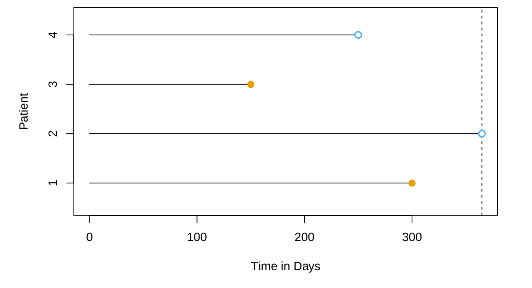
For each individual, we suppose that there is a true failure or event time T, as well as a true censoring time C.
The survival time represents the time at which the event of interest occurs (such as death).
By contrast, the censoring is the time at which censoring occurs: for example, the time at which the patient drops out of the study or the study ends.
We observe either the survival time T or else the censoring time C. Specifically, we observe the random variable Y = min(T,C) \qquad \tag{1}
If the event occurs before censoring (i.e. T < C) then we observe the true survival time T; if censoring occurs before the event (T > C) then we observe the censoring time. We also observe a status indicator, \delta = \begin{cases} 1 & \text{if } T \leq C, \\ 0 & \text{if } T > C. \end{cases} \qquad \tag{2}
Finally, in our dataset we observe n pairs (Y,δ), which we denote as (y_1,δ_1),\ldots, (y_n,δ_n).
- Survival and Censoring Times
- Defines true survival time (T) and true censoring time (C).
- Explains the observed time (Y) as the minimum of T and C.
- Introduces the status indicator (δ) to differentiate between observed event time and censoring time.
A Closer Look at Censoring
Suppose that a number of patients drop out of a cancer study early because they are very sick.
An analysis that does not take into consideration the reason why the patients dropped out will likely overestimate the true average survival time.
Similarly, suppose that males who are very sick are more likely to drop out of the study than females who are very sick. Then a comparison of male and female survival times may wrongly suggest that males survive longer than females.
In general, we need to assume that, conditional on the features, the event time T is independent of the censoring time C. The two examples above violate the assumption of independent censoring.
A Closer Look at Censoring
- Discusses the assumption of independent censoring.
- Explains right censoring and mentions other censoring types such as left censoring and interval censoring.
The Kaplan–Meier Survival Curve

- The Survival Curve
The survival function (or curve) is defined as S(t) = Pr(T > t) \qquad \tag{3}
This decreasing function quantifies the probability of surviving past time t.
For example, suppose that a company is interested in modeling customer churn. Let T represent the time that a customer cancels a subscription to the company’s service.
Then S(t) represents the probability that a customer cancels later than time t. The larger the value of S(t), the less likely that the customer will cancel before time t
- Estimating the Survival Curve
- Consider the BrainCancer dataset, which contains the survival times for patients with primary brain tumors undergoing treatment with stereotactic radiation methods.
- The predictors are gtv (gross tumor volume, in cubic centimeters); sex (male or female); diagnosis (meningioma, LG glioma, HG glioma, or other); loc (the tumor location: either infratentorial or supratentorial); ki (Karnofsky index); and stereo (stereotactic method).
- Only 53 of the 88 patients were still alive at the end of the study.
- Suppose we’d like to estimate S(20) = Pr(T > 20), the probability that a patient survives for at least 20 months,
- It is tempting to simply compute the proportion of patients who are known to have survived past 20 months, that is, the proportion of patients for whom Y > 20.
- This turns out to be 48/88, or approximately 55%.
- However, this does not seem quite right: 17 of the 40 patients who did not survive to 20 months were actually censored, and this analysis implicitly assumes they died before 20 months. Hence it is probably an underestimate
- The Kaplan–Meier Survival Curve
- Defines the survival curve (survival function) S(t).
- Presents the Kaplan-Meier estimator for estimating the survival curve in the presence of censoring.
- Illustrates the Kaplan-Meier survival curve using the BrainCancer dataset.
The Log-Rank Test

- Females seem to fare a little better up to about 50 months, but then the two curves both level off to about 50%. How can we carry out a formal test of equality of the two survival curves?
- At first glance, a two-sample t-test seems like an obvious choice: but the presence of censoring again creates a complication.
- To overcome this challenge, we will conduct a log-rank test.
- Recall that d1 < d2 < ···< dK are the unique death times among the non-censored patients, rk is the number of patients at risk at time dk, and qk is the number of patients who died at time dk.
- We further define r_{1k} and r_{2k} to be the number of patients in groups 1 and 2, respectively, who are at risk at time d_k.
- Similarly, we define q_{1k} and q_{2k} to be the number of patients in groups 1 and 2, respectively, who died at time d_k. Note that r_{1k} + r_{2k} = rk and q_{1k} + q_{2k} = q_k.
Details of the Test Statistic:
| Group 1 | Group 2 | Total | |
|---|---|---|---|
| Died | q_{1k} | q_{2k} | q_k |
| Survived | r_{1k} − q_{1k} | r_{2k} − q_{2k} | r_k − q_k |
| Total | r_{1k} | r_{2k} | r_k |
- The log-rank test statistic is given by At each death time dk, we construct a 2 ×2 table of counts of the form shown above.
- Note that if the death times are unique (i.e. no two individuals die at the same time), then one of q_{1k} and q_{2k} equals one, and the other equals zero.
Log Rank Test: the Main Idea
To test H_0 : \mathbb{E}[X] = 0 for some random variable X, one approach is to construct a test statistic of the form: W = \frac{X-\mathbb{E}[X]}{\sqrt{\text{Var}(X)}} \qquad \tag{4}
where \mathbb{E}[X] and Var(X) are the expectation and variance, respectively, of X under H_0.
In order to construct the log-rank test statistic, we compute a quantity that takes exactly the form above, with X = \sum_{k=1}^K q_{1k}, where q_{1k} is given in the top left of the table above.
The Final Result
The resulting formula for the log-rank test statistic is: W = \frac{\sum_{k=1}^K (q_{1k}- \mathbb{E}(q_{1k}) )}{\sqrt{ \sum_{k=1}^K Var (q_{1k})}} = \frac{\sum_{k=1}^K (q_{1k}- \frac{q_k}{r_k} r_{1k})}{\sqrt{ \sum_{k=1}^K \frac{q_k}{(r_k-1)} (r_{1k}/r_k)(1-r_{1k}/r_k)(r_k-q_k)}} \qquad \tag{5}
When the sample size is large, the log-rank test statistic W has approximately a standard normal distribution.
This can be used to compute a p-value for the null hypothesis that there is no difference between the survival curves in the two groups.
The Log-Rank Test
- Explains the log-rank test for comparing survival curves between two groups.
- Details the construction of the log-rank test statistic based on a contingency table of event counts at each unique death time.
- Shows the application of the log-rank test on the BrainCancer data to compare survival
Regression Models With a Survival Response
We now consider the task of fitting a regression model to survival data.
We wish to predict the true survival time T. Since the observed quantity Y = min(T,C) is positive and may have a long right tail, we might be tempted to fit a linear regression of log(Y ) on X. But censoring again creates a problem.
To overcome this difficulty, we instead make use of a sequential construction, similar to the idea used for the Kaplan-Meier survival curve.
Regression Models With a Survival Response
- Discusses the challenge of fitting regression models to survival data with censoring.
- Introduces the hazard function as an alternative approach to modeling survival times.
The Hazard Function
Defines the hazard function h(t) and its relationship to the survival function S(t) and probability density function f(t).
The hazard function or hazard rate — also known as the force of mortality — is formally defined as h(t) = \lim_{\Delta t \rightarrow 0} \frac{Pr(t < T \le t + \Delta t \mid T > t)}{\Delta t} \qquad \tag{6}
where T is the (true) survival time.
It is the death rate in the instant after time t, given survival up to that time.
The hazard function is the basis for the Proportional Hazards Model.
Discusses the likelihood function for survival data with censoring.
Explains the limitation of assuming a specific functional form for the hazard function.
Proportional Hazards

- Presents the proportional hazards assumption and explains the baseline hazard.
h(t\mid x_i) = h_0(t) exp \left( \sum_{j=1}^p x_{ij} \beta_j \right) \qquad \tag{7}
- Where h_0(t) ≥ 0 is an unspecified function, known as the baseline hazard. It is the hazard function for an individual with features x_{i1} = \ldots = x_{ip} = 0.
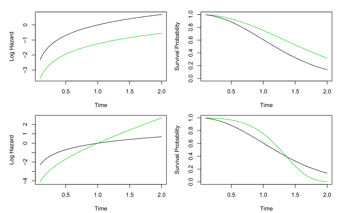
Bottom: Again we have a single binary covariate x_i \in {0, 1}. However, the proportional hazards assumption (11.14) does not hold. The log hazard functions cross, as do the survival functions.
- Introduces Cox’s proportional hazards model for estimating regression coefficients without specifying the baseline hazard.
- The name proportional hazards arises from the fact that the hazard function for an individual with feature vector x_i is some unknown function h_0(t) times the factor exp \left( \sum_{j=1}^p x_{ij} \beta_j \right). . The quantity exp \left( \sum_{j=1}^p x_{ij} \beta_j \right) is called the relative risk for the feature vector x_i = (x_{i1}, \ldots, x_{ip}), relative to that for the feature vector x_i = (0, \ldots, 0).
- The Cox model estimates the regression coefficients \beta_1, \ldots, \beta_p by maximizing a partial likelihood function. This function is the product of the probabilities of the observed events, and it does not require specification of the baseline hazard function h_0(t).
- What does it mean that the baseline hazard function h_0(t) is unspecified?
- Basically, we make no assumptions about its functional form. We allow the instantaneous probability of death at time t, given that one has survived at least until time t, to take any form.
- This means that the hazard function is very flexible and can model a wide range of relationships between the covariates and survival time.
- Our only assumption is that a one-unit increase in x_{ij} corresponds to an increase in h(t \mid x_i) by a factor of exp(β_j).
- Discusses the partial likelihood and its importance in Cox’s model.
- Highlights the connection between the log-rank test and Cox’s model with a single binary covariate.
Example: Brain Cancer Data
- Applies Cox’s proportional hazards model to the BrainCancer data.
- Interprets the estimated coefficients and their statistical significance.
Example: Publication Data
- Analyzes the Publication data using Kaplan-Meier curves and Cox’s proportional hazards model.
- Discusses the effect of positive results on time to publication after adjusting for other covariates.
Shrinkage for the Cox Model
In this section of the book the authors consider use of shrinkage method developed in section 6.2. to the Cox model. where they are motivated by the “loss+penalty” formulation of Section 6.2, we consider minimizing a penalized version of the negative log partial likelihood .
This seems interesting if one whishes to formulate this as a hierarchical model, where shrinkage of coefficents is a common propertty of the models.
- log \left( \prod_{i : \delta_i=1} \frac{ exp (\sum_{j=1}^p x_{ij}\beta_j) }{\sum_{i'} exp (\sum_{i ': y_i'>y_i}^p x_{i'j}\beta_j) } \right ) + \gamma P(\beta) \qquad
- Introduces penalized Cox models with ridge and lasso penalties.
- Applies the lasso-penalized Cox model to the Publication data and interprets the cross-validation results.
- Demonstrates the use of risk scores for assessing model fit on the test set.
Additional Topics
- Briefly covers additional topics in survival analysis:
- AUC and Harrell’s concordance index for evaluating survival models.
- Choice of time scale.
- Time-dependent covariates and their application in Cox’s model.
- Methods for checking the proportional hazards assumption.
- Survival trees and random survival forests as extensions of tree-based methods.
Area Under the Curve for Survival Analysis
This is an appealing method for assessing a fitted Cox model on a test set.
For each observation, we calculate the estimated risk score, using the estimated Cox model coefficients via: \hat{η}_i = \hat{β}_1 x_{i1} + \ldots + \hat{β}_px_{ip}, for i = 1, \ldots , n \tag{8}
Then Harrell’s concordance index (or C-index) computes the proportion of observation pairs for which \hat{\eta}_{i'} > \hat{\eta}_{i} and \hat{y}_{i'} >\hat{y}_{i}
C = \frac{\sum_{i,i'} \mathbb{I}(\hat{\eta}_{i'} > \hat{\eta}_i) \delta_{i'}}{\sum_{i,i'} \delta_{i'}} \qquad \tag{9}
- where \mathbb{I}(·) is the indicator function, which equals 1 if the argument is true and 0 otherwise.
- This is the proportion of pairs for which the model correctly predicts the relative survival time, among all pairs for which this can be determined
Choice of Time Scale
- One of the challenges of survival analysis and any temporal model is the choice of time scale. In many case it is possible to derive many features from the time dimension.
- For censoring there is an added complexity though in the sense that we may want to shift different cohorts to begin at the same relative time.
- This is a common problem in churn prediction where we may want to compare the survival of different cohorts.
- In this section the authors discuss subtleties involved in the choice of zero time (enrolment) and failure time (event time)
- In epidemiology, one may set time zero to the patient’s birth removing the need to adjust for age in the analysis.
- If there is a treatment - the time of treatment may be a natural zero time.
- In reality I don’t think that the authors have provided a clear answer to this question, but rather opened a can of worms.
Time-Dependent Covariates
- A powerful feature of the proportional hazards model is its ability to handle time-dependent covariates, predictors whose value may change over time.
- Because the partial likelihood in (11.16) is constructed sequentially in time, dealing with time-dependent covariates is straightforward
- The idea is that we might to encode a feature as f(x,t) rather than f(x) in the model to indicate the predictor is time dependent and more succictly that f(x) has a value at time t.
Checking the Proportional Hazards Assumption
The Cox model depends on the assumption that the hazard ratio between two individuals is constant over time. While the model is robust to mild violations of this assumption, it is worthwhile to test it.
Survival Trees
- Survival trees are a modification of classification and regression trees that use a split criterion that maximizes the difference between the survival curves in the resulting daughter nodes.
- Survival trees can then be used to create random survival forests.
- C.f. (Bou-Hamad, Larocque, and Ben-Ameur 2011) A review of survival trees
Lab: Survival Analysis
- Provides hands-on examples of survival analysis using Python libraries.
Brain Cancer Data
- Application to the Brain Cancer Dataset is here
- Analyzes the BrainCancer and Publication datasets using Kaplan-Meier curves, log-rank tests, and Cox’s proportional hazards model.
- Comparing the survival times of females and males on the BrainCancer data gives a log-rank test statistic of W = 1.2, which corresponds to a two-sided p-value of 0.2.
- Thus, we cannot reject the null hypothesis of no difference in survival curves between females and males.
- The log-rank test is closely related to Cox’s proportional hazards model, which we discuss next.
Publication Data
Call Center Data
- Simulates call center data and analyzes the wait times with survival analysis techniques.
- See here
Exercises
References
Further Reading
Software for Survival Analysis:
- The examples in this lecture were creating using the survival and glmnet packages in R.
- Both packages can handle time-dependent covariates and general forms of censoring.
- Software for other machine learning approaches can be found both the R repository and the scikit-survival Python collection.
Wikipedia Articles:
Books
- Survival Analysis: A Self-Learning Text by David G. Kleinbaum and Mitchel Klein
- Applied Survival Analysis: Regression Modeling of Time-to-Event Data by David W. Hosmer, Jr., Stanley Lemeshow, and Susanne May
- Applied Survival Analysis Using R by Dirk F. Moore
- Survival Analysis: Techniques for Censored and Truncated Data by John P. Klein and Melvin L. Moeschberger
Papers:
- Kaplan, E. L., & Meier, P. (1958). Nonparametric estimation from incomplete observations. Journal of the American statistical association, 53(282), 457-481.
- Cox, D. R. (1972). Regression models and life-tables. Journal of the Royal Statistical Society. Series B (Methodological), 34(2), 187-220.
- Asymptotically Efficient Rank Invariant Test Procedures by Richard Peto and Julian Peto is the source of the log-rank test.
- Lin, D. Y., Wei, L. J., & Ying, Z. (1993). Checking the Cox model with cumulative sums of martingale-based residuals. Biometrika, 80(3), 557-572.
- Therneau, T. M., & Grambsch, P. M. (2000). Modeling survival data: extending the Cox model. Springer Science & Business Media.
Additional Readings:
- The Kumaraswamy Weibull distribution: A generalization of the Weibull probability distribution by Gauss M. Cordeiro, Edwin M. M. Ortega, Marcelino A. de Pascoa
- A Nonidentifiability Aspect of the Problem of Competing Risks by Anastasios A. Tsiatis
Slides
Chapter
References
Reuse
Citation
@online{bochman2024,
  author = {Bochman, Oren},
  title = {Chapter 11: {Survival} {Analysis} and {Censored} {Data}},
  date = {2024-09-01},
  url = {https://orenbochman.github.io/notes-islr/posts/ch11/},
  langid = {en}
}