Chapter 12: Unsupervised Learning – An Introduction to Statistical Learning

Figure 1: Principal Components

Figure 2: Higher order principal components

Figure 3: k-means clustering

Figure 4: Hierarchical Clustering

Figure 5: Matrix Completion

Figure 6: Breast Cancer Example

Figure 7: Principal Components

Figure 8: K-means Clustering

Figure 9: Hierarchical Clustering

TL;DR - Unsupervised Learning

Unsupervised Learning Learning in a nutshell

Principal Component Analysis (PCA) is an unsupervised learning approach that involves only a set of features X_1, X_2, \ldots, X_p measured on n observations. PCA is not interested in prediction. Instead, the goal is to discover interesting things about the measurements. PCA can be used for data visualization, data pre-processing before supervised learning, and data imputation.
Matrix Completion is a method for imputing missing data that uses principal components. It can be used if the data is missing at random (i.e., the reason the value is missing is not related to the value itself). Matrix completion is used in recommender systems.

Chapter Orientation

This chapter contains some big words, but don’t worry, we’ll break them down together.

Principal Component Analysis (PCA): An unsupervised learning approach that involves only a set of features X_1, X_2, \ldots, X_p measured on n observations. PCA is not interested in prediction. Instead, the goal is to discover interesting things about the measurements. PCA can be used for data visualization, data pre-processing before supervised learning, and data imputation.
Principal Components: Normalized linear combinations of features that have the largest variance Each principal component is uncorrelated with the others.
Loadings: The elements (\phi_{11}, \phi_{21}, ... \phi_{p1}) of the principal component loading vector \phi_{11}.
Loading Vector: A vector made up of the loadings \phi_1=(\phi_{11}, \phi_{21}, ... \phi_{p1})^T. The loading vector defines the direction in feature space along which the data vary the most.
Principal Component Scores: The values that result from projecting the n data points X_1, X_2, \ldots, X_p onto the direction defined by the loading vector. They can be represented by z₁₁, …, z_n1.
Biplot: A plot that displays both the principal component scores and the loading vectors.
Proportion of Variance Explained (PVE): The proportion of variance in a data set that is explained by a principal component. The PVE can be interpreted as the R² of the approximation for X given by the first M principal components.
Scree Plot: A plot that depicts the proportion of variance explained by each of the principal components. It can be used to decide how many principal components are needed.
Imputation: Filling in missing values in a data matrix.
Matrix Completion: A method for imputing missing data that uses principal components. It can be used if the data is missing at random (i.e., the reason the value is missing is not related to the value itself). Matrix completion is used in recommender systems.
Recommender Systems: Systems that use matrix completion to predict a user’s preferences. They predict a user’s rating for an item by leveraging their past behavior and the preferences of similar users.
Clustering: A set of techniques used to find subgroups in a data set without having an associated response variable Y. Clustering is an unsupervised method because it attempts to discover structure (i.e., distinct clusters) on the basis of a data set.
K-means Clustering: A clustering method that partitions the data into a pre-specified number of clusters (K).
Hierarchical Clustering: A clustering method that does not require knowing the number of clusters in advance. It results in a dendrogram, which allows for simultaneous viewing of clusters obtained for each possible number of clusters (from 1 to n).
Dendrogram: A tree-like visualization of the observations that results from hierarchical clustering. The height of the cut on the dendrogram serves the same role as the K in K-means clustering, and determines the number of clusters obtained.
Bottom-up (Agglomerative) Clustering: The most common type of hierarchical clustering. The dendrogram (typically depicted as an upside-down tree) is built by combining clusters starting from the leaves and going up to the trunk.
Linkage: The definition of dissimilarity between two groups of observations. It extends the concept of dissimilarity between a pair of observations to a pair of groups of observations. The four most common types of linkage are complete, average, single, and centroid.
Inversion: This occurs in centroid linkage, where two clusters are fused at a height below either of the individual clusters in the dendrogram. Inversions can make dendrograms difficult to interpret.

Chapter Outline

Unsupervised learning uses statistical tools to discover information about a set of features X₁, X₂, …, X_p measured on n observations. Unlike supervised learning methods, unsupervised learning methods are not used for prediction because they are not applied to a response variable Y. The goal of unsupervised learning is to explore and understand the relationships and patterns within the features. Unsupervised learning can answer questions like:

How can data be visualized informatively?
Can subgroups be found among variables or observations?

Some techniques in unsupervised learning include principal components analysis and clustering.

Applications of Unsupervised Learning

Unsupervised learning is used in various fields, including:

Cancer research: Researchers can use gene expression levels in patients with breast cancer to identify subgroups among patients or genes. This provides a better understanding of the disease.
E-commerce: Online retailers can identify groups of shoppers with similar buying habits. This enables them to show each shopper items that they are more likely to buy based on the purchase history of similar shoppers.

Principal Components Analysis

Principal components analysis (PCA) is a technique used for:

Data visualization
Data pre-processing before using supervised techniques
Data imputation (filling in missing values)

What are Principal Components?

Principal components (PCs) are a way to find a low-dimensional representation of a dataset that captures most of its variation. Each PC is a linear combination of the original features.

Imagine a dataset with n observations and p features. PCA finds a smaller number of dimensions that represent the most variation in the data, allowing the information to be visualized.

How are Principal Components Found?

PCA finds the linear combination of features, called Z₁, with the largest sample variance. This linear combination is subject to a constraint that ensures the sum of the squares of the coefficients (loadings) equals one.

The first principal component loading vector (a direction in feature space) represents the direction in which the data varies the most. Projecting the n data points onto this direction gives the principal component scores.

After determining the first PC, subsequent PCs are found in a similar way, but they are constrained to be uncorrelated with the previous PCs. This constraint means that each new PC direction is orthogonal (perpendicular) to the previous directions.

Proportion of Variance Explained

It’s natural to ask how much information is lost when projecting the observations onto a smaller number of PCs. The proportion of variance explained (PVE) by each PC quantifies this information loss.

The PVE can be interpreted as the R² of the approximation for the data matrix X using the first M principal components.

Importance of Scaling

Scaling the variables before performing PCA is generally recommended. If variables are measured in different units or have vastly different variances, scaling ensures that each variable contributes equally to the PCs. This prevents PCs from being dominated by variables with the largest variance.

Deciding How Many Principal Components to Use

There are several methods to determine the optimal number of PCs:

Scree Plot: A scree plot visualizes the PVE of each component. The “elbow” point in the plot, where the proportion of variance explained drops off, is often chosen as the cutoff for the number of PCs.
Supervised Analysis: When using PCA for supervised learning, cross-validation can be used to determine the optimal number of PC score vectors to use as features.
Subjective Evaluation: If using PCA for data exploration, the choice is subjective. It’s common to examine the first few PCs and continue until no further interesting patterns are found.

Other Uses for Principal Components

Principal components can be used as features in various statistical techniques, such as regression, classification, and clustering. Using the PC score vectors instead of the full data matrix can lead to less noisy results. This is because the signal in the data is often concentrated in the first few PCs.

Missing Values and Matrix Completion

Missing values in datasets can be a problem for statistical analyses. Matrix completion is a technique that uses PCA to impute missing values by exploiting the correlation between variables. This is only applicable if the data is missing at random (MAR). For example, missing a patient’s weight because the scale’s battery died is an example of MAR. However, if the weight is missing because the patient was too heavy for the scale, it is not MAR, and matrix completion would not be suitable.

Principal Components with Missing Values

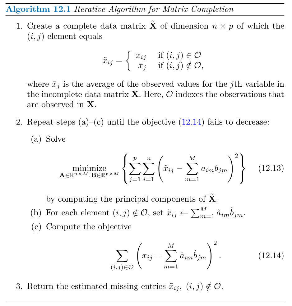
Matrix completion seeks to find the principal component score and loading vectors that best approximate the observed data matrix. This involves minimizing the sum of squared differences between the observed data and its approximation based on the PC score and loading vectors.

Once the problem is solved, the missing values can be imputed using the estimated score and loading vectors.

Algorithm 12.1 provides an iterative method for imputing missing values and solving the principal component problem simultaneously. The algorithm initializes a complete data matrix by replacing missing values with column means. It then iteratively updates the missing values by approximating the matrix using the first M principal components until the error is minimized.

Clustering Methods

Clustering methods are used to group observations in a dataset into subgroups, or clusters, such that observations within a cluster are similar to each other and different from observations in other clusters. The definition of similarity is often specific to the domain and the data being studied.

For example, a cancer researcher might use clustering to find subgroups of patients with breast cancer based on gene expression measurements. The idea is that different subtypes of breast cancer may exist, and clustering can help discover them.

Types of Clustering

Two common types of clustering methods are:

K-means clustering: This method partitions the data into a pre-specified number of clusters (K).
Hierarchical clustering: This method does not require specifying the number of clusters beforehand. It produces a tree-like representation of the observations called a dendrogram. The dendrogram shows the clusterings obtained for all possible numbers of clusters, from 1 to n.

K-means Clustering

K-means clustering aims to partition data into K distinct, non-overlapping clusters by minimizing the within-cluster variation.

Algorithm 12.2 outlines the K-means clustering procedure:

Randomly assign each observation to one of the K clusters.
Iterate until the cluster assignments stabilize:
- Calculate the cluster centroid (the vector of feature means) for each cluster.
- Reassign each observation to the cluster with the closest centroid (using Euclidean distance).

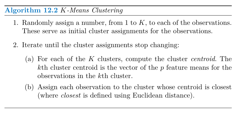
Algorithm 12.2 is guaranteed to find a local optimum for the K-means optimization problem. The algorithm iteratively improves the clustering by minimizing the sum-of-squared deviations within each cluster.

One challenge with K-means clustering is that the algorithm can converge to different local optima depending on the initial random cluster assignments. To address this, the algorithm can be run multiple times with different initial configurations, and the solution with the lowest objective value is selected.

Hierarchical Clustering

Hierarchical clustering is an alternative approach that doesn’t require pre-specifying the number of clusters. It creates a dendrogram that visually represents the observations’ hierarchical relationships.

Agglomerative clustering, a bottom-up approach, is the most common type of hierarchical clustering. It starts with each observation as its own cluster and iteratively merges the most similar clusters until all observations belong to a single cluster.

Interpreting a Dendrogram

A dendrogram’s leaves represent individual observations. As you move up the tree, branches fuse, indicating the merging of similar observations or clusters. The height of the fusion on the vertical axis represents the dissimilarity between the groups being merged.

It’s important to note that the horizontal axis in a dendrogram doesn’t represent similarity. The dendrogram can be reordered without changing its meaning, so the proximity of observations on the horizontal axis is not indicative of their similarity.

Clusters can be identified by making a horizontal cut across the dendrogram. The sets of observations below the cut represent distinct clusters.

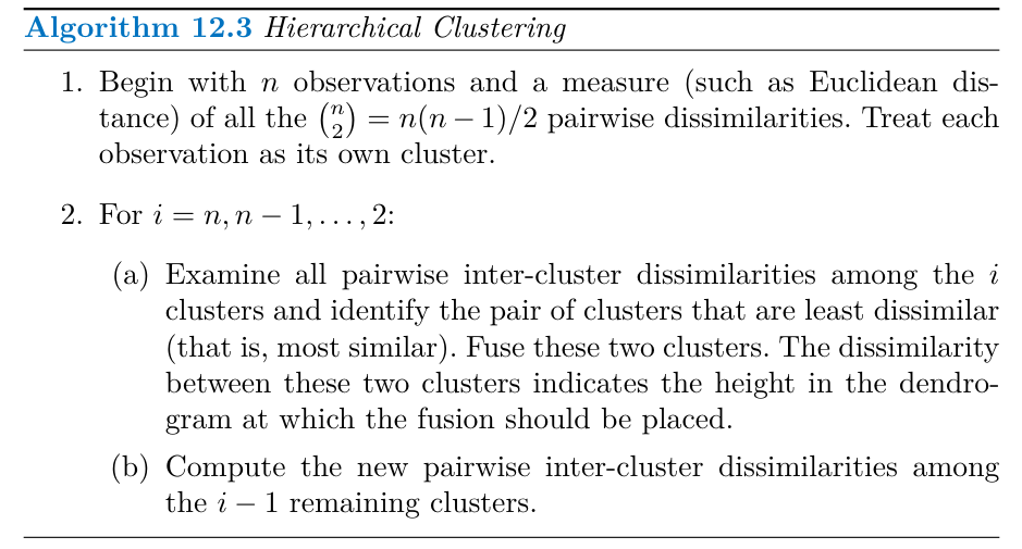
The Hierarchical Clustering Algorithm

Algorithm 12.3 outlines the hierarchical clustering procedure:

Start with n observations as individual clusters and calculate all pairwise dissimilarities.
Iteratively, for i from n down to 2:
- Find the two clusters with the smallest dissimilarity and merge them.
- Update the pairwise dissimilarities between the remaining clusters.

Linkage

Linkage defines the dissimilarity between two groups of observations and significantly influences the hierarchical clustering results. Common linkage types include:

Complete linkage: Uses the maximum dissimilarity between observations in the two clusters.
Single linkage: Uses the minimum dissimilarity between observations in the two clusters. This method can lead to extended, trailing clusters, where observations are added one by one.
Average linkage: Uses the average dissimilarity between observations in the two clusters.
Centroid linkage: Uses the dissimilarity between the centroids of the two clusters. This method can lead to inversions in the dendrogram, which can make interpretation difficult.

Average and complete linkage are generally preferred over single linkage because they produce more balanced dendrograms.

Choice of Dissimilarity Measure

The choice of dissimilarity measure can affect the clustering results. Euclidean distance is common, but other measures like correlation-based distance can be more appropriate depending on the context.

Correlation-based distance considers observations similar if their feature values are highly correlated, even if the Euclidean distance is large. This measure is useful when the shape of the observation profiles is more important than their absolute values.

Practical Issues in Clustering

There are several practical considerations when using clustering methods:

Standardization: The choice of whether and how to standardize the data can impact the results.
Choice of Parameters: The dissimilarity measure, linkage type (in hierarchical clustering), the number of clusters (K in K-means clustering), and the dendrogram cut height all need to be chosen carefully.
Cluster Validation: Evaluating whether the clusters found reflect true subgroups or just noise is important. While methods exist to assess the statistical significance of clusters, there is no single best approach.
Outliers: Forcing every observation into a cluster can distort the results if outliers exist. Techniques like mixture models can handle outliers more effectively.
Robustness: Clustering results can be sensitive to data perturbations. It’s recommended to cluster subsets of the data to understand the robustness of the findings.

It’s crucial to interpret clustering results with caution and consider them as a starting point for further investigation rather than definitive conclusions. Repeating the analysis with different parameter settings and data subsets can provide a more comprehensive understanding of the data.

The sources provide a lab demonstration of applying PCA and clustering in Python, including code examples for:

Performing PCA on the USArrests data.
Implementing matrix completion.
Performing K-means and hierarchical clustering on a simulated dataset.
Analyzing the NCI60 cancer cell line microarray data using PCA and hierarchical clustering.

Excercises

Conceptual

This problem involves the K-means clustering algorithm.
1. Prove (12.18).
2. On the basis of this identity, argue that the K-means clustering algorithm (Algorithm 12.2) decreases the objective (12.17) at each iteration.
Suppose that we have four observations, for which we compute a dissimilarity matrix, given by
\begin{bmatrix} 0& 0.3& 0 .4& 0 .7& \\ 0.3& 0& .5& 0.8\\ 0.4& 0.5& 0& .45\\ 0.7 &0.8& 0.45&0\end{bmatrix}

For instance, the dissimilarity between the first and second observations is 0.3, and the dissimilarity between the second and fourth observations is 0.8.
1. On the basis of this dissimilarity matrix, sketch the dendrogram that results from hierarchically clustering these four observations using complete linkage. Be sure to indicate on the plot the height at which each fusion occurs, as well as the observations corresponding to each leaf in the dendrogram.
2. Repeat (a), this time using single linkage clustering.
3. Suppose that we cut the dendrogram obtained in (a) such that two clusters result. Which observations are in each cluster?
4. Suppose that we cut the dendrogram obtained in (b) such that two clusters result. Which observations are in each cluster?
5. It is mentioned in this chapter that at each fusion in the dendrogram, the position of the two clusters being fused can be swapped without changing the meaning of the dendrogram. Draw a dendrogram that is equivalent to the dendrogram in (a), for which two or more of the leaves are repositioned, but for which the meaning of the dendrogram is the same.

Obs.	X1	X2
1	1	4
2	1	3
3	0	4
4	5	1
5	6	2
6	4	0

In this problem, you will perform K-means clustering manually, with K = 2 , on a small example with n = 6 observations and p = 2 features. The observations are above.
1. Plot the observations.
2. Randomly assign a cluster label to each observation. You can use the np.random.choice() function to do this. Report the cluster labels for each observation.
3. Compute the centroid for each cluster.
4. Assign each observation to the centroid to which it is closest, in terms of Euclidean distance. Report the cluster labels for each observation.
5. Repeat (c) and (d) until the answers obtained stop changing.
6. In your plot from (a), color the observations according to the cluster labels obtained.
Suppose that for a particular data set, we perform hierarchical clustering using single linkage and using complete linkage. We obtain two dendrograms.
1. At a certain point on the single linkage dendrogram, the clusters {1, 2, 3}and {4, 5} fuse. On the complete linkage dendro- gram, the clusters {1, 2, 3}and {4, 5} also fuse at a certain point. Which fusion will occur higher on the tree, or will they fuse at the same height, or is there not enough information to tell?
2. At a certain point on the single linkage dendrogram, the clusters {5}and {6} fuse. On the complete linkage dendrogram, the clusters {5}and {6}also fuse at a certain point. Which fusion will occur higher on the tree, or will they fuse at the same height, or is there not enough information to tell?
In words, describe the results that you would expect if you performed K-means clustering of the eight shoppers in Figure 12.16, on the basis of their sock and computer purchases, with K = 2 . Give three answers, one for each of the variable scalings displayed. Explain. 554 12. Unsupervised Learning
We saw in Section 12.2.2 that the principal component loading and score vectors provide an approximation to a matrix, in the sense of (12.5). Specifically, the principal component score and loading vectors solve the optimization problem given in (12.6). Now, suppose that the M principal component score vectors zim, m = 1, . . . , M , are known. Using (12.6), explain that each of the first M principal component loading vectors φjm, m = 1 , . . . , M , can be ob- tained by performing p separate least squares linear regressions. In each regression, the principal component score vectors are the predictors, and one of the features of the data matrix is the response. Applied
In this chapter, we mentioned the use of correlation-based distance and Euclidean distance as dissimilarity measures for hierarchical clus- tering. It turns out that these two measures are almost equivalent: if each observation has been centered to have mean zero and standard deviation one, and if we let rij denote the correlation between the ith and jth observations, then the quantity 1 −rij is proportional to the squared Euclidean distance between the ith and jth observations. On the US Arrests data, show that this proportionality holds. Hint: The Euclidean distance can be calculated using the pairwise_distances() function from the sklearn.metrics module, and pairwise_ distances()correlations can be calculated using the np.corrcoef() function.
In Section 12.2.3, a formula for calculating PVE was given in Equa- tion 12.10. We also saw that the PVE can be obtained using the explained_variance_ratio_ attribute of a fitted PCA() estimator. On the USArrests data, calculate PVE in two ways:
1. Using the explained_variance_ratio_ output of the fitted PCA() estimator, as was done in Section 12.2.3.
2. By applying Equation 12.10 directly. The loadings are stored as the components_ attribute of the fitted PCA() estimator. Use those loadings in Equation 12.10 to obtain the PVE. These two approaches should give the same results. Hint: You will only obtain the same results in (a) and (b) if the same data is used in both cases. For instance, if in (a) you performed PCA() using centered and scaled variables, then you must center and scale the variables before applying Equation 12.10 in (b).
Consider the USArrests data. We will now perform hierarchical clus- tering on the states.
1. Using hierarchical clustering with complete linkage and Euclidean distance, cluster the states.
2. Cut the dendrogram at a height that results in three distinct clusters. Which states belong to which clusters?
3. Hierarchically cluster the states using complete linkage and Eu- clidean distance, after scaling the variables to have standard deviation one.
4. What effect does scaling the variables have on the hierarchical clustering obtained? In your opinion, should the variables be scaled before the inter-observation dissimilarities are computed? Provide a justification for your answer.
In this problem, you will generate simulated data, and then perform PCA and K-means clustering on the data.
1. Generate a simulated data set with 20 observations in each of three classes (i.e. 60 observations total), and 50 variables. Hint: There are a number of functions in Python that you can use to generate data. One example is the normal() method of the random() function in numpy; the uniform() method is another option. Be sure to add a mean shift to the observations in each class so that there are three distinct classes.
2. Perform PCA on the 60 observations and plot the first two prin- cipal component score vectors. Use a different color to indicate the observations in each of the three classes. If the three classes appear separated in this plot, then continue on to part (c). If not, then return to part (a) and modify the simulation so that there is greater separation between the three classes. Do not continue to part (c) until the three classes show at least some separation in the first two principal component score vectors.
3. Perform K-means clustering of the observations with K = 3 . How well do the clusters that you obtained in K-means cluster- ing compare to the true class labels? Hint: You can use the pd.crosstab() function in Python to compare the true class labels to the class labels obtained by cluster- ing. Be careful how you interpret the results: K-means clustering will arbitrarily number the clusters, so you cannot simply check whether the true class labels and clustering labels are the same.
4. Perform K-means clustering with K = 2 . Describe your results.
5. Now perform K-means clustering with K = 4 , and describe your results.
6. Now perform K-means clustering with K = 3 on the first two principal component score vectors, rather than on the raw data. That is, perform K-means clustering on the 60 × 2 matrix of which the first column is the first principal component score vector, and the second column is the second principal component score vector. Comment on the results.
7. Using the StandardScaler() estimator, perform K-means clustering with K = 3 on the data after scaling each variable to have standard deviation one. How do these results compare to those obtained in (b)? Explain.
Write a Python function to perform matrix completion as in Algorithm 12.1, and as outlined in Section 12.5.2. In each iteration, the function should keep track of the relative error, as well as the itera- tion count. Iterations should continue until the relative error is small enough or until some maximum number of iterations is reached (set a default value for this maximum number). Furthermore, there should be an option to print out the progress in each iteration. Test your function on the Boston data. First, standardize the features to have mean zero and standard deviation one using the StandardScaler() function. Run an experiment where you randomly leave out an increasing (and nested) number of observations from 5% to 30%, in steps of 5%. Apply Algorithm 12.1 with M = 1 , 2, . . . , 8. Display the approximation error as a function of the fraction of ob- servations that are missing, and the value of M , averaged over 10 repetitions of the experiment.
In Section 12.5.2, Algorithm 12.1 was implemented using the svd() function from the np.linalg module. However, given the connection between the svd() function and the PCA() estimator highlighted in the lab, we could have instead implemented the algorithm using PCA(). Write a function to implement Algorithm 12.1 that makes use of PCA() rather than svd().
On the book website, www.statlearning.com there is a gene expression data set (Ch12Ex13.csv) that consists of 40 tissue samples with measurements on 1,000 genes. The first 20 samples are from healthy patients, while the second 20 are from a diseased group.
1. Load in the data using pd.read_csv(). You will need to select header = None.
2. Apply hierarchical clustering to the samples using correlation-based distance, and plot the dendrogram. Do the genes separate the samples into the two groups? Do your results depend on the type of linkage used?
3. Your collaborator wants to know which genes differ the most across the two groups. Suggest a way to answer this question, and apply it here.

Slides

Chapter Slides

Chapter

Reuse

CC SA BY-NC-ND

Citation

BibTeX citation:

@online{bochman2024,
  author = {Bochman, Oren},
  title = {Chapter 12: {Unsupervised} {Learning}},
  date = {2024-09-10},
  url = {https://orenbochman.github.io/notes-islr/posts/ch12/},
  langid = {en}
}

For attribution, please cite this work as:

Bochman, Oren. 2024. “Chapter 12: Unsupervised Learning.” September 10, 2024. https://orenbochman.github.io/notes-islr/posts/ch12/.