Opening Remarks
Examples and Framework
- 9 Support Vector Machines
- 9.1 Maximal Margin Classifier
- 9.1.1 What Is a Hyperplane?
- 9.1.2 Classification Using a Separating Hyperplane
- 9.1.3 The Maximal Margin Classifier
- 9.1.4 Construction of the Maximal Margin Classifier
- 9.1.5 The Non-separable Case
- 9.2 Support Vector Classifiers
- 9.2.1 Overview of the Support Vector Classifier
- 9.2.2 Details of the Support Vector Classifier
- 9.3 Support Vector Machines
- 9.3.1 Classification with Non-Linear Decision Boundaries
- 9.3.2 The Support Vector Machine
- 9.3.3 An Application to the Heart Disease Data
- 9.4 SVMs with More than Two Classes
- 9.4.1 One-Versus-One Classification
- 9.4.2 One-Versus-All Classification
- 9.5 Relationship to Logistic Regression
- 9.6 Lab: Support Vector Machines
- 9.6.1 Support Vector Classifier
- 9.6.2 Support Vector Machine
- 9.6.3 ROC Curves
- 9.6.4 SVM with Multiple Classes
- 9.6.5 Application to Gene Expression Data
- 9.7 Exercises
SVM are cool. I never used them very much as most problems involve more than two classes and the extension are not as easy to understand as other methods of multivariate classification.
However SVM are very popular and also useful for intuition. about data. Kernels are a very powerful concept and will arise in gaussian processes and many other methods.

- Maximal Margin Classifier: The SVM finds the hyperplane that maximizes the margin between classes.
- Support Vector Classifier: The SVM allows for misclassification by introducing slack variables.
- Support Vector Machine: The SVM extends to nonlinear decision boundaries using kernels.
- KKT Conditions: The Karush-Kuhn-Tucker conditions are necessary for the SVM solution.
- Soft Margin: The SVM can handle noisy data by allowing for misclassification.
- Multi-Class SVM: The SVM can be extended to more than two classes.
- Hyperplane
- A flat affine subspace of dimension p-1 in a p-dimensional space, used as a decision boundary.
- Separating Hyperplane
- A hyperplane that perfectly divides the training data into distinct classes.
- Maximal Margin Classifier
- A linear classifier that finds the separating hyperplane with the largest margin (distance to the nearest data points).
- Margin
- The perpendicular distance between the maximal margin hyperplane and the closest training observations (support vectors).
- Support Vectors
- The training data points that lie closest to the decision boundary and directly influence the position and orientation of the maximal margin hyperplane or support vector classifier.
- Support Vector Classifier
- An extension of the maximal margin classifier that allows for some misclassifications (soft margin) to handle non-separable data.
- Slack Variable
- A variable introduced in the support vector classifier’s optimization problem to allow training observations to violate the margin or the hyperplane.
- Tuning Parameter (C)
- A non-negative parameter in the support vector classifier that controls the trade-off between maximizing the margin and minimizing the training error (number of margin violations).
- Feature Expansion
- The process of transforming the original features into a higher-dimensional space by adding non-linear functions or combinations of the original features.
- Kernel
- A function that quantifies the similarity between two data points and implicitly computes the inner product in a potentially high-dimensional feature space without explicitly performing the transformation.
- Linear Kernel
- A kernel function that computes the standard dot product between two feature vectors, resulting in a linear decision boundary.
- Polynomial Kernel
- A kernel function that uses a polynomial of the features to compute similarity, enabling non-linear decision boundaries of a polynomial form.
- Radial Kernel (RBF)
- A kernel function that measures similarity based on the distance between data points, often using an exponential decay, allowing for complex, non-linear decision boundaries.
- Kernel Trick
- The technique of using kernel functions in SVMs to operate in high-dimensional spaces efficiently without explicitly computing the coordinates of the data in that space.
- One-Versus-One (OVO)
- A strategy for multi-class classification using SVMs by training a binary classifier for every pair of classes.
- One-Versus-All (OVA) / One-Versus-Rest
- A strategy for multi-class classification using SVMs by training a binary classifier for each class against all other classes.
- Hinge Loss
- The loss function used in the formulation of the support vector classifier, which penalizes misclassified points and points within the margin on the wrong side.
- Support Vector Machine (SVM)
- A powerful supervised learning algorithm for classification (and regression) that extends the support vector classifier by using kernel methods to handle non-linear decision boundaries.
- Support Vector Regression
- An extension of SVMs to handle regression problems with a focus on minimizing errors outside a certain margin.
- Decision Function
- The function learned by an SVM that outputs a real value for a given input, whose sign determines the predicted class label.
- ROC Curve (Receiver Operating Characteristic Curve)
- A graphical plot that illustrates the diagnostic ability of a binary classifier as its discrimination threshold is varied.
The following are some of the functions and methods used in the code:
RocCurveDisplay.from_estimator()- A function in scikit-learn used to plot ROC curves from a fitted estimator.
SupportVectorClassifier() / SVC()- A function in scikit-learn used to implement support vector classification.
decision_function()- A method of a fitted SVM estimator in scikit-learn that returns the decision function values for the input data.
confusion_table()- A function (from the ISLP package) that displays the confusion matrix, showing the counts of true positives, true negatives, false positives, and false negatives.
SupportVectorRegression()- A function in scikit-learn used to implement support vector regression.
GridSearchCV()- A function in scikit-learn used for systematic hyperparameter tuning by searching over a specified parameter grid and evaluating performance using cross-validation.
KFold()- A cross-validation iterator in scikit-learn that provides train/test indices to split data in k consecutive folds.
Outline
Support Vector Machines (SVMs) are a powerful and popular approach for classification, developed in the 1990s. They are particularly effective for high-dimensional data and have gained popularity in various fields, including bioinformatics, text classification, and image recognition.
The key idea behind SVMs is to find a hyperplane that separates the data points of different classes with the maximum margin.
In the podcast we use a couple of analogies like separating potato chips from pretzels which is what seems to be going on when we look at a svm on a scatterplot.
The other analogy is a fence between rival fans in a football game. Here we would like to keep the fans of the two teams apart with a margin separating them. The wider the margin the better. If we cant actually separate the fans we would like the fence to have as many fans on the right sides as possible.
- Introduction and Overview of Support Vector Machines:
The authors introduce SVMs as a powerful and popular approach for classification. In the chapter they notes that SVMs
“have been shown to perform well in a variety of settings, and are often considered one of the best ‘out of the box’ classifiers.”
In the slides they frame the approach as directly tackling the two-class classification problem by finding a separating plane in feature space, and then getting creative by
“soften[ing] what we mean by ‘separates’” and “enrich[ing] and enlarge[ing] the feature space so that separation is possible.”
They distinguishing between the maximal margin classifier in (Section 9.1), the support vector classifier (Section 9.2), and the support vector machine (Section 9.3), emphasizing the importance of careful distinction to avoid common confusion.
Hyperplanes as Decision Boundaries: (Section 9.1.2)
The authors define a hyperplane as a flat affine subspace of dimension p–1 in a p-dimensional space.
In two dimensions, it’s a line, and in three dimensions, it’s a plane.
The mathematical definition of a hyperplane is given by the linear equation:
β_0 + β_1 X_1 + β_2 X_2 + · · ·+ β_p X_p = 0 \qquad \tag{1}
The sources explain that a hyperplane divides the p-dimensional space into two halves. The sign of the expression β_0 + β_1 X_1 + · · ·+ β_p X_p for a given point X determines which side of the hyperplane it lies on. This forms the basis for classification: a test observation is assigned a class based on which side of the separating hyperplane it falls.
we can see how this happens mathematically
point lying off the line satisfy either:
β_0 + β_1 X_1 + β_2 X_2 + · · ·+ β_p X_p > 0 \qquad \tag{2} or
β_0 + β_1 X_1 + β_2 X_2 + · · ·+ β_p X_p < 0 \qquad \tag{3}
So we understand the geometry of the hyperplane used as a decision boundary, but we still need to understand how to learn the parameters β_0, β_1, · · ·, β_p. that gives us the best decision boundary.
Maximal Margin Classifier – the Optimal Separator (Section 9.1.3)
The chapter introduces the maximal margin classifier as a natural choice when the classes are linearly separable. It highlights that while “there will in fact exist an infinite number of such hyperplanes,” the maximal margin hyperplane (also known as the optimal separating hyperplane) is the one that is “farthest from the training observations.”
The margin is defined as the smallest perpendicular distance from any of the training observations to the hyperplane. The maximal margin classifier aims to maximize this margin.
“The maximal margin hyperplane is the separating hyperplane for which the margin is largest—that is, it is the hyperplane that has the farthest minimum distance to the training observations.”
The slides visually and mathematically represent this constrained optimization problem, aiming to maximize M (the margin) subject to the constraints that all data points are correctly classified and at least a distance M from the hyperplane.
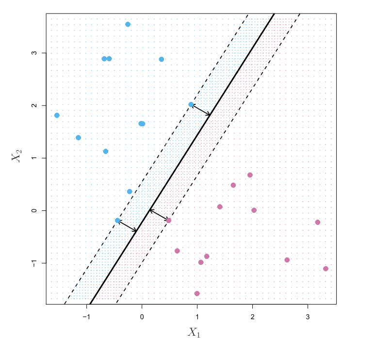
Support Vectors: The chapter introduces the concept of support vectors as the training observations that lie on the boundary of the margin (the dashed lines in Figure 1). These points are crucial because “if these points were moved slightly then the maximal margin hyperplane would move as well.” The classifier depends directly on these support vectors and not on other observations further away from the boundary.
The authors both point out a significant limitation of the maximal margin classifier: it requires the classes to be perfectly separable by a linear boundary, which is a hard assumption to make for any real-world datasets.
Additionally, even with separable data, it can be sensitive to noisy data and outliers, potentially leading to overfitting (as illustrated in Figure 9.5 in the chapter).
Given these two problems we would like to have a more flexible approach that allows for some misclassification and is less sensitive to outliers.
- Support Vector Classifier: Allowing for Errors (Soft Margin):
To address the issue of non-separable data and sensitivity to outliers, the chapter introduces the support vector classifier. This is an extension that allows for some training observations to be misclassified or to lie within the margin. This is achieved by introducing slack variables (ε_i in the slides, ξ_i conceptually similar to ε_i in the context of the chapter though denoted differently in the optimization problem).
The optimization problem for the support vector classifier (Equation 9.12-9.15 in the chapter) aims to maximize the margin while penalizing violations using these slack variables. The tuning parameter C (or λ inversely related in the hinge loss formulation) controls the trade-off between maximizing the margin and minimizing the number of margin violations.
“As the budget C increases, we become more tolerant of violations to the margin, and so the margin will widen. Conversely, as C decreases, we become less tolerant of violations to the margin and so the margin narrows.” (chapter)
The slides also illustrates this with varying values of C, showing how the decision boundary and margin change. Importantly, similar to the maximal margin classifier, the decision boundary of the support vector classifier is still linear in the original feature space, and the classifier is still determined by support vectors (observations that lie on or violate the margin).
- Support Vector Machines: Handling Non-Linear Boundaries with Kernels:
To tackle problems with non-linear class boundaries, authors introduce the support vector machine (SVM). The key idea is to enlarge the feature space by using non-linear transformations of the original features. A support vector classifier is then fit in this higher-dimensional space, resulting in a non-linear decision boundary in the original space.
The computationally efficient way to achieve this feature space enlargement is through the use of kernels. A kernel function K(x_i, x_{i'}) quantifies the similarity between two observations and can be thought of as an inner product in the enlarged feature space without explicitly computing the transformations.
“The support vector machine (SVM) is an extension of the support vector classifier that results from enlarging the feature space in a specific way, using kernels.” (book)
“If we can compute inner-products between observations, we can fit a SV classifier. Can be quite abstract! Some special kernel functions can do this for us.” (slides)
Some examples of common kernel functions:
Linear Kernel:
K(x_i, x_{i'}) = \sum^p_{j=1} x_{ji}x_{i'j}
(simply the standard inner product, equivalent to the support vector classifier). Polynomial Kernel: K(x_i, x_{i'}) = (1 + \sum^p_{j=1} x_{ij}x_{i'j})^d
(allows for polynomial decision boundaries of degree d). Radial Kernel (RBF): K(xi, xi’) = exp(-γ ∑ (xji - x’ji)^2) (creates more flexible, potentially local decision boundaries, where γ controls the influence of nearby points). The solution for an SVM with a kernel takes the form:
f(x) = β_0 + \sum_{i\in S} \hat{\alpha_i} K(x, x_i)
where S is the set of support vectors.
The chapter highlights that using kernels avoids the computational burden of explicitly working in the potentially very high or even infinite-dimensional enlarged feature space.
9.4 SVMs for More Than Two Classes:
We briefly discuss extending SVMs to handle multi-class classification (K > 2 classes). Two common approaches are mentioned:
One-Versus-All (OVA) / One-Versus-Rest (OVR): Train K binary SVM classifiers, each comparing one class against all the others. A new observation is assigned to the class whose classifier outputs the highest confidence score.
One-Versus-One (OVO): Train K(K-1)/2 binary SVM classifiers, one for each pair of classes. A new observation is classified based on a voting scheme, where it’s assigned to the class that wins the most pairwise competitions. The slides suggest that OVO is preferred if K is not too large.
- Relationship to Logistic Regression:
The (Section 9.5) discusses the close connections between SVMs and other statistical methods like logistic regression. It shows that the support vector classifier optimization can be rewritten in a “Loss + Penalty” form:
minimize β_0,β_1,...,β_p { \sum \max [0, 1− y if(x_i)] + λ \sum β^2_j } \text{(hinge loss + L2 penalty)}
The loss function used in SVMs is the hinge loss, which is compared to the loss function used in logistic regression (negative log-likelihood) in Figure 9.12 (“ch09.pdf”). The hinge loss is exactly zero for observations correctly classified beyond the margin, contributing to the sparsity of the solution (reliance on support vectors). While the logistic loss is never exactly zero, it becomes very small for well-classified points.
The comparison:
When classes are nearly separable, SVMs tend to perform better than logistic regression. When classes overlap more significantly, logistic regression (often with a ridge penalty) and SVMs often yield similar results.
If probability estimates are required, logistic regression is the preferred choice. Kernel SVMs are popular for non-linear boundaries, and while kernels can be used with logistic regression and LDA, the computations can be more expensive.
- Practical Implementation (from Lab Section):
The lab section demonstrates the use of the SVC() function from the sklearn.svm library in Python. It covers:
Fitting linear SVMs with different values of the cost parameter C and observing the impact on the decision boundary and support vectors.
Handling linearly separable and non-linearly separable data. Using non-linear kernels (“poly” and “rbf”) and tuning their parameters (degree, gamma, and C) using cross-validation (GridSearchCV).
Generating and interpreting ROC curves using RocCurveDisplay.from_estimator() and the decision_function() method to evaluate classifier performance at different thresholds. Briefly illustrating multi-class classification with decision_function_shape.
Applying a linear SVM to a high-dimensional gene expression dataset (Khan data), noting the suitability of a linear kernel when the number of features is much larger than the number of observations.
Slides and Chapter
Reuse
Citation
@online{bochman2024,
  author = {Bochman, Oren},
  title = {Chapter 9: {Support} {Vector} {Machines}},
  date = {2024-08-10},
  url = {https://orenbochman.github.io/notes-islr/posts/ch09/},
  langid = {en}
}