Chapter 2: Introduction to Python - Lab Graphics

Graphics

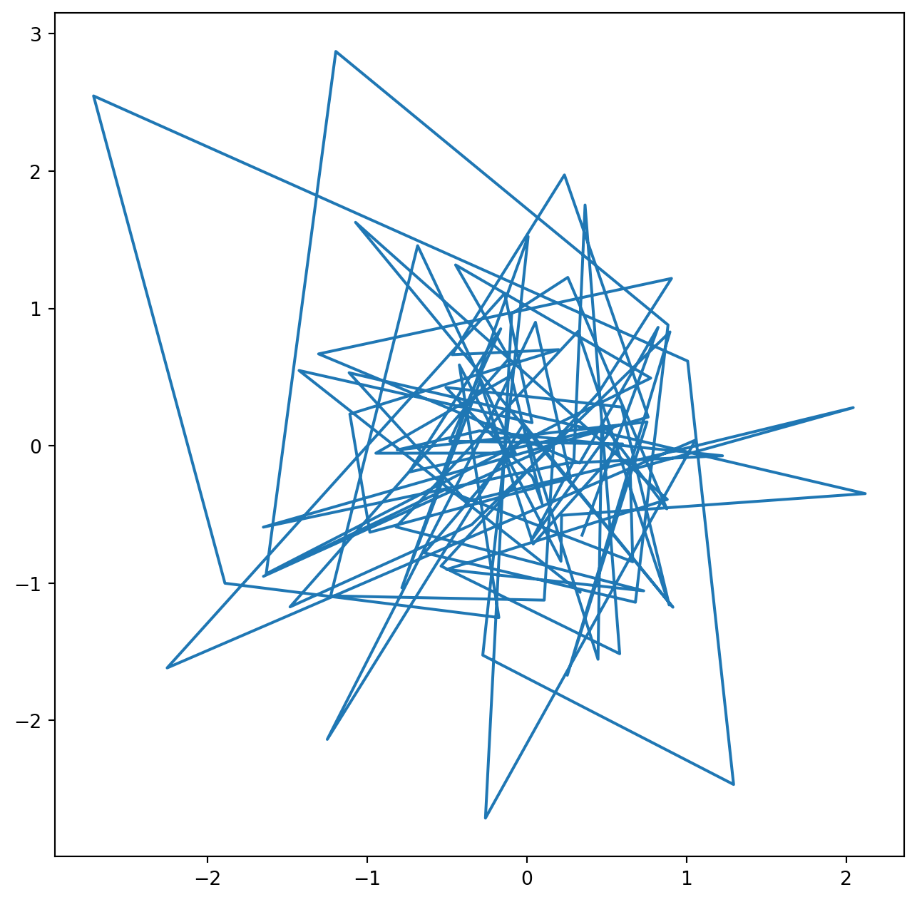
In Python, common practice is to use the library matplotlib for graphics. However, since Python was not written with data analysis in mind, the notion of plotting is not intrinsic to the language. We will use the subplots() function from matplotlib.pyplot to create a figure and the axes onto which we plot our data. For many more examples of how to make plots in Python, readers are encouraged to visit matplotlib.org/stable/gallery/.

In matplotlib, a plot consists of a figure and one or more axes. You can think of the figure as the blank canvas upon which one or more plots will be displayed: it is the entire plotting window. The axes contain important information about each plot, such as its x- and y-axis labels, title, and more. (Note that in matplotlib, the word axes is not the plural of axis: a plot’s axes contains much more information than just the x-axis and the y-axis.)

We begin by importing the subplots() function from matplotlib. We use this function throughout when creating figures. The function returns a tuple of length two: a figure object as well as the relevant axes object. We will typically pass figsize as a keyword argument. Having created our axes, we attempt our first plot using its plot() method. To learn more about it, type ax.plot?.

import numpy as np 
import pandas as pd
from matplotlib.pyplot import subplots

rng = np.random.default_rng(1)

fig, ax = subplots(figsize=(8, 8))
x = rng.standard_normal(100)
y = rng.standard_normal(100)
ax.plot(x, y);

We pause here to note that we have unpacked the tuple of length two returned by subplots() into the two distinct variables fig and ax. Unpacking is typically preferred to the following equivalent but slightly more verbose code:

output = subplots(figsize=(8, 8))
fig = output[0]
ax = output[1]

We see that our earlier cell produced a line plot, which is the default. To create a scatterplot, we provide an additional argument to ax.plot(), indicating that circles should be displayed.

fig, ax = subplots(figsize=(8, 8))
ax.plot(x, y, 'o');

Different values of this additional argument can be used to produce different colored lines as well as different linestyles.

As an alternative, we could use the ax.scatter() function to create a scatterplot.

fig, ax = subplots(figsize=(8, 8))
ax.scatter(x, y, marker='o');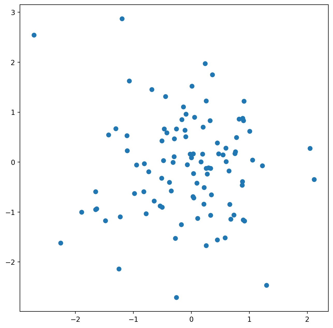

Notice that in the code blocks above, we have ended the last line with a semicolon. This prevents ax.plot(x, y) from printing text to the notebook. However, it does not prevent a plot from being produced. If we omit the trailing semi-colon, then we obtain the following output:

fig, ax = subplots(figsize=(8, 8))
ax.scatter(x, y, marker='o')

In what follows, we will use trailing semicolons whenever the text that would be output is not germane to the discussion at hand.

To label our plot, we make use of the set_xlabel(), set_ylabel(), and set_title() methods of ax.

fig, ax = subplots(figsize=(8, 8))
ax.scatter(x, y, marker='o')
ax.set_xlabel("this is the x-axis")
ax.set_ylabel("this is the y-axis")
ax.set_title("Plot of X vs Y");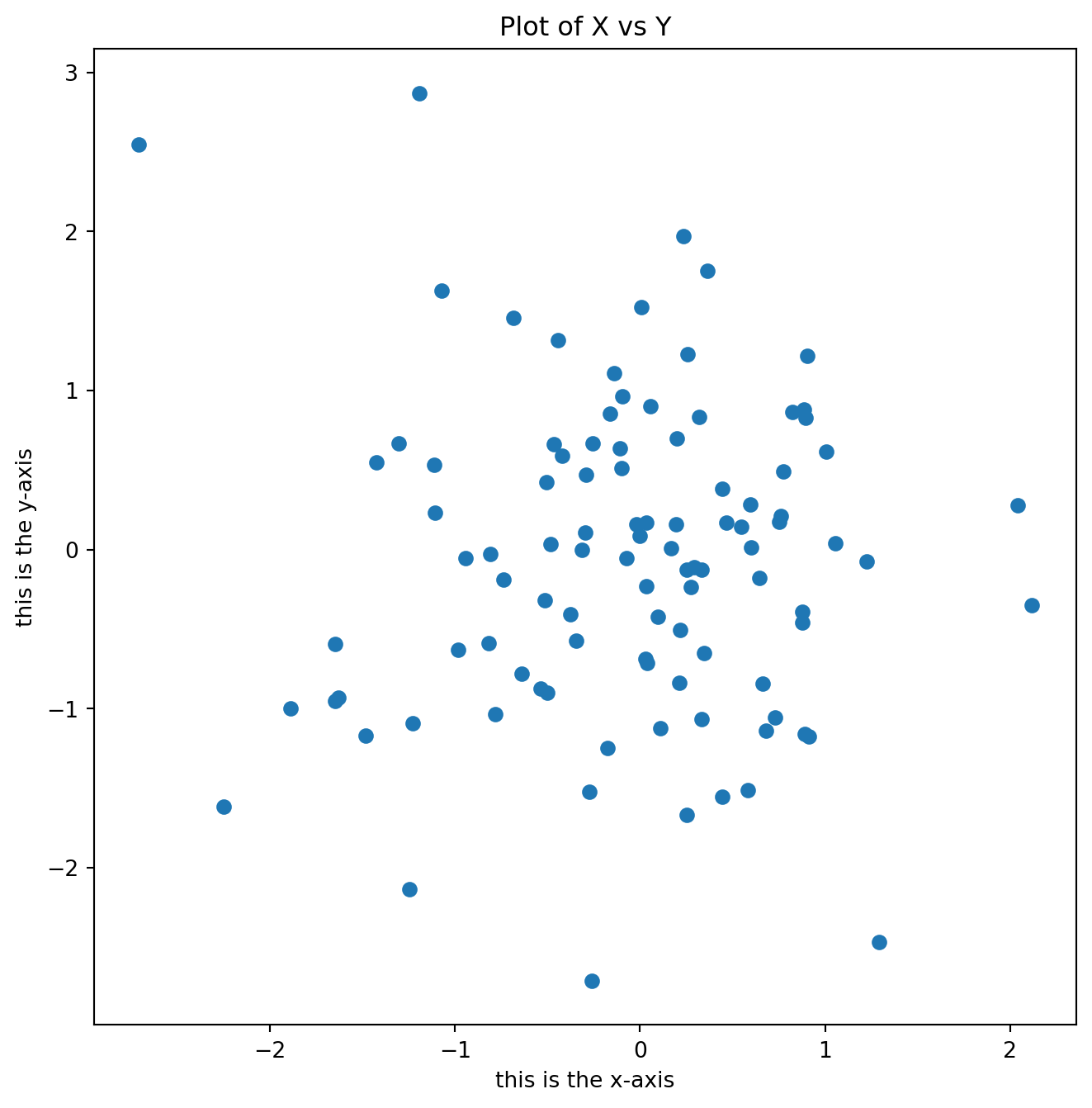

Having access to the figure object fig itself means that we can go in and change some aspects and then redisplay it. Here, we change the size from (8, 8) to (12, 3).

fig.set_size_inches(12,3)
fig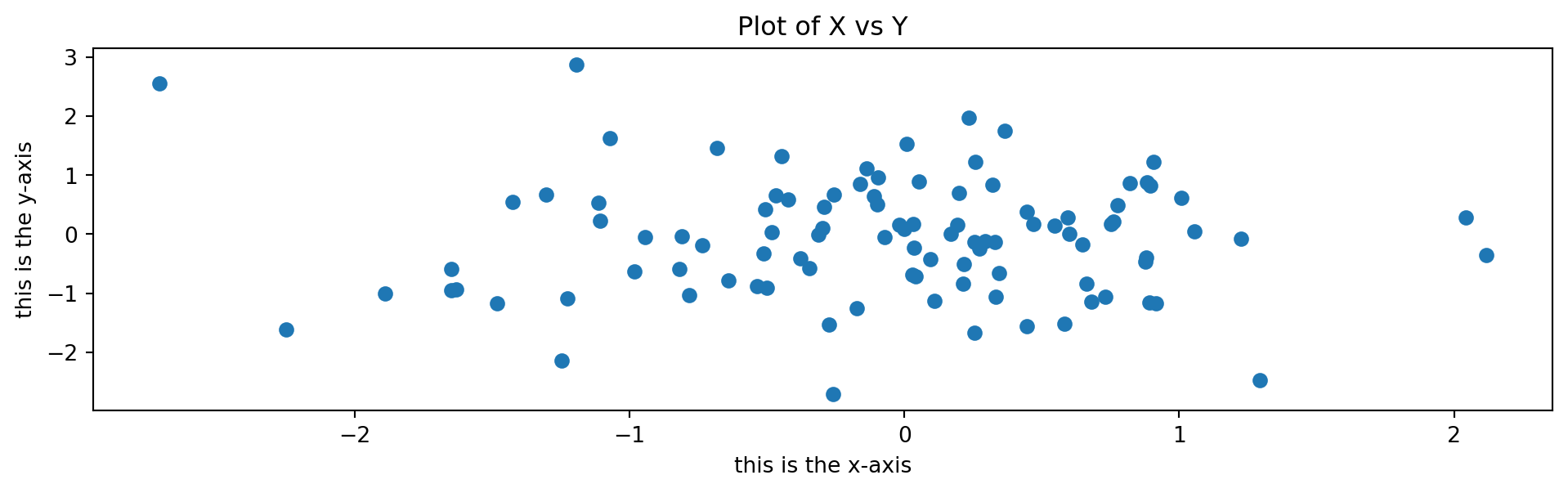

Occasionally we will want to create several plots within a figure. This can be achieved by passing additional arguments to subplots(). Below, we create a 2 \times 3 grid of plots in a figure of size determined by the figsize argument. In such situations, there is often a relationship between the axes in the plots. For example, all plots may have a common x-axis. The subplots() function can automatically handle this situation when passed the keyword argument sharex=True. The axes object below is an array pointing to different plots in the figure.

fig, axes = subplots(nrows=2,
                     ncols=3,
                     figsize=(15, 5))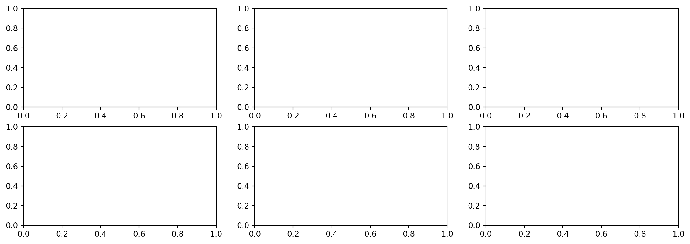

We now produce a scatter plot with 'o' in the second column of the first row and a scatter plot with '+' in the third column of the second row.

axes[0,1].plot(x, y, 'o')
axes[1,2].scatter(x, y, marker='+')
fig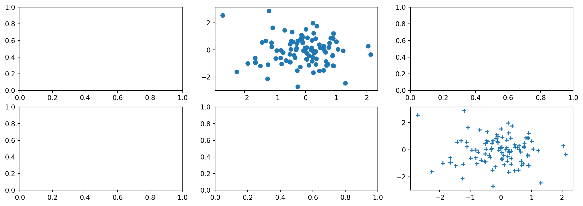

Type subplots? to learn more about subplots().

To save the output of fig, we call its savefig() method. The argument dpi is the dots per inch, used to determine how large the figure will be in pixels.

fig.savefig("Figure.png", dpi=400)
fig.savefig("Figure.pdf", dpi=200);

We can continue to modify fig using step-by-step updates; for example, we can modify the range of the x-axis, re-save the figure, and even re-display it.

axes[0,1].set_xlim([-1,1])
fig.savefig("Figure_updated.jpg")
fig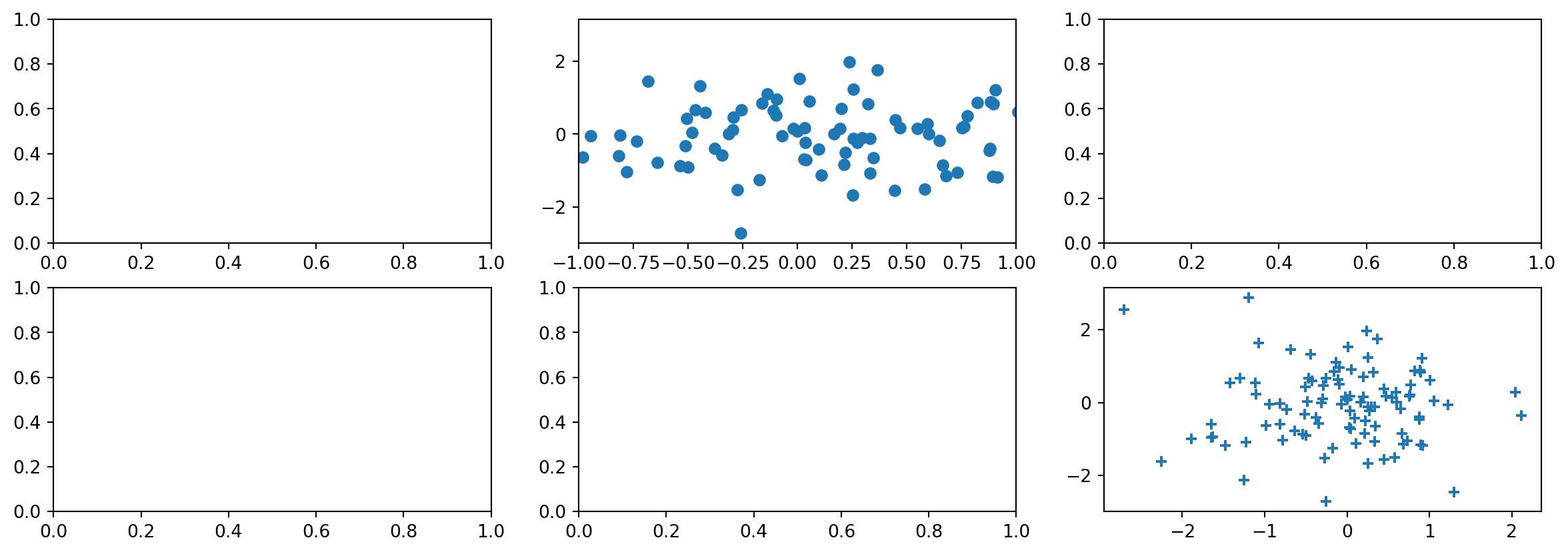

We now create some more sophisticated plots. The ax.contour() method produces a contour plot in order to represent three-dimensional data, similar to a topographical map. It takes three arguments:

• A vector of x values (the first dimension),
• A vector of y values (the second dimension), and
• A matrix whose elements correspond to the z value (the third dimension) for each pair of (x,y) coordinates.

To create x and y, we’ll use the command np.linspace(a, b, n), which returns a vector of n numbers starting at a and ending at b.

fig, ax = subplots(figsize=(8, 8))
x = np.linspace(-np.pi, np.pi, 50)
y = x
f = np.multiply.outer(np.cos(y), 1 / (1 + x**2))
ax.contour(x, y, f);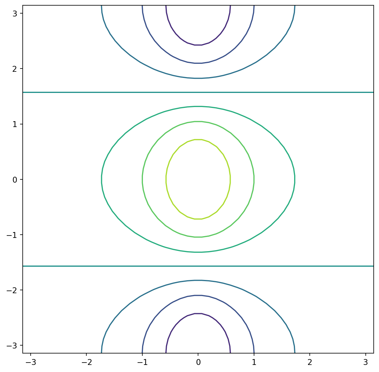

We can increase the resolution by adding more levels to the image.

fig, ax = subplots(figsize=(8, 8))
ax.contour(x, y, f, levels=45);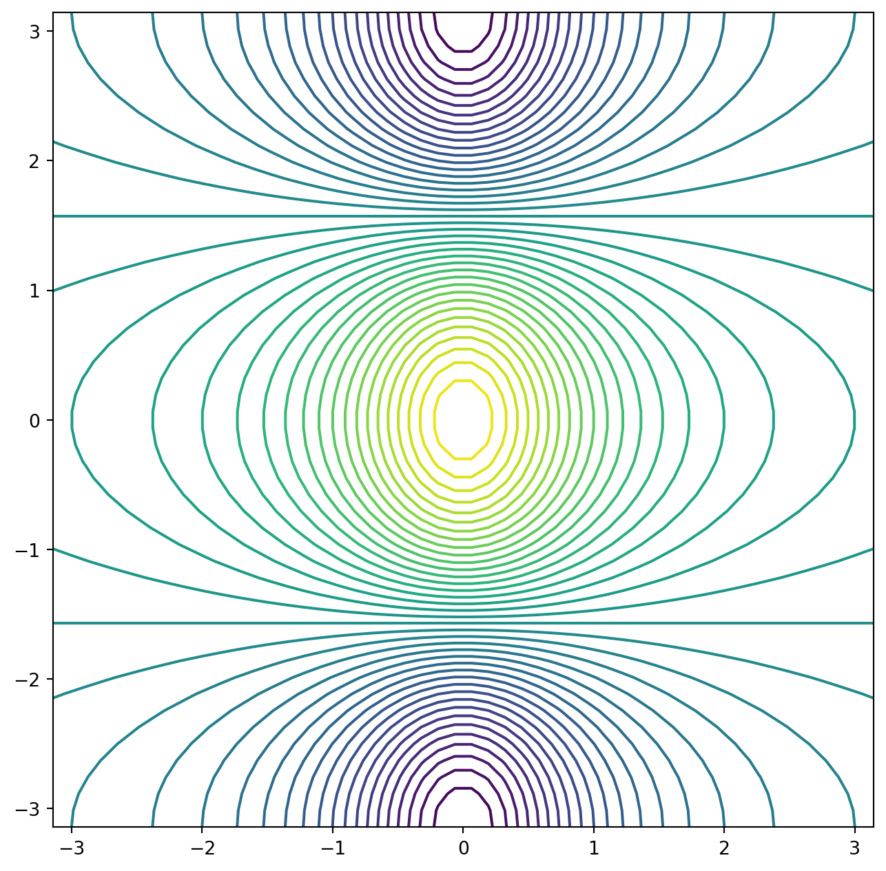

To fine-tune the output of the ax.contour() function, take a look at the help file by typing ?plt.contour.

The ax.imshow() method is similar to ax.contour(), except that it produces a color-coded plot whose colors depend on the z value. This is known as a heatmap, and is sometimes used to plot temperature in weather forecasts.

fig, ax = subplots(figsize=(8, 8))
ax.imshow(f);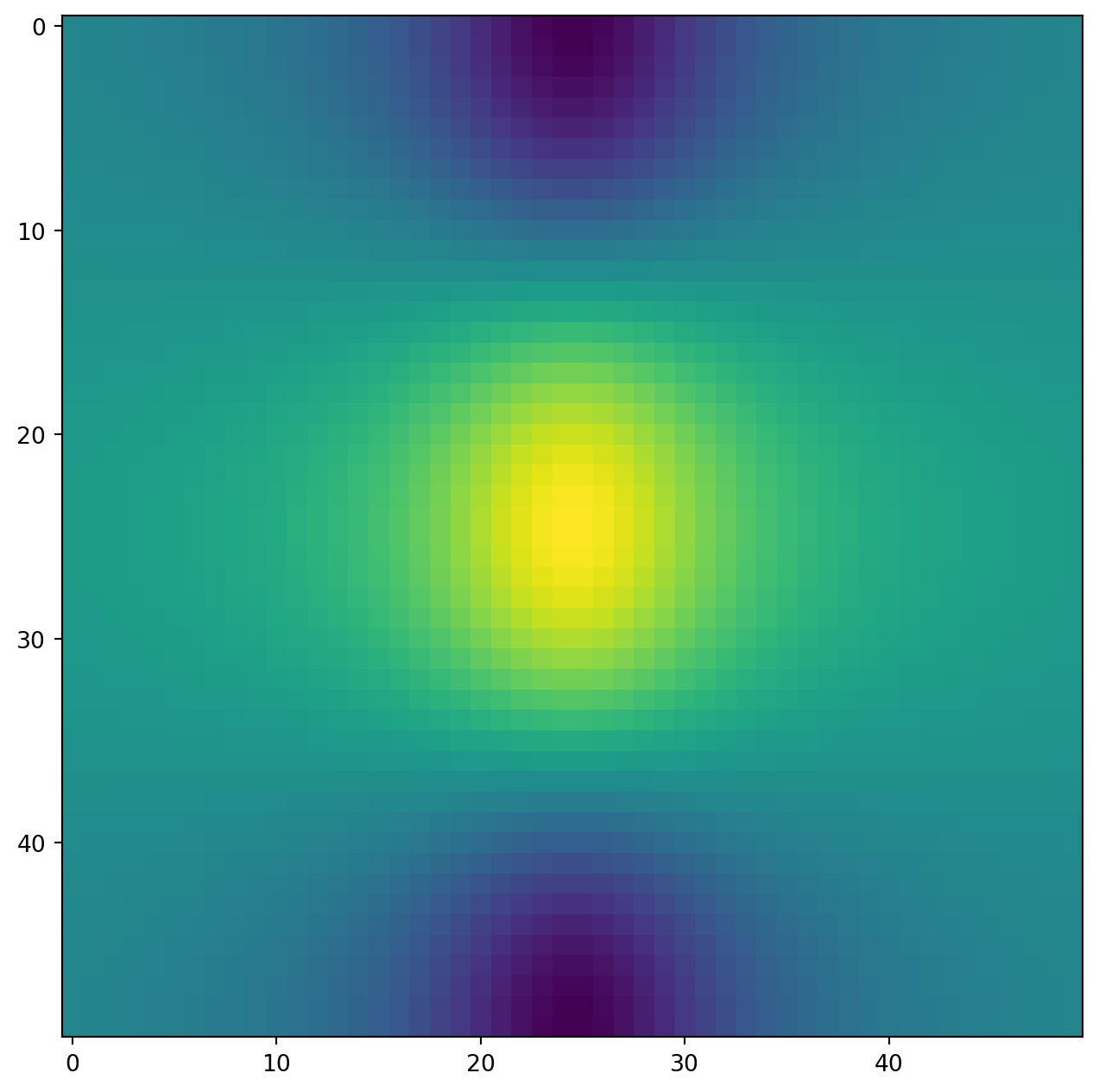

Sequences and Slice Notation

As seen above, the function np.linspace() can be used to create a sequence of numbers.

seq1 = np.linspace(0, 10, 11)
seq1

array([ 0.,  1.,  2.,  3.,  4.,  5.,  6.,  7.,  8.,  9., 10.])

The function np.arange() returns a sequence of numbers spaced out by step. If step is not specified, then a default value of 1 is used. Let’s create a sequence that starts at 0 and ends at 10.

seq2 = np.arange(0, 10)
seq2

array([0, 1, 2, 3, 4, 5, 6, 7, 8, 9])

Why isn’t 10 output above? This has to do with slice notation in Python. Slice notation
is used to index sequences such as lists, tuples and arrays. Suppose we want to retrieve the fourth through sixth (inclusive) entries of a string. We obtain a slice of the string using the indexing notation [3:6].

"hello world"[3:6]

'lo '

In the code block above, the notation 3:6 is shorthand for slice(3,6) when used inside [].

"hello world"[slice(3,6)]

'lo '

You might have expected slice(3,6) to output the fourth through seventh characters in the text string (recalling that Python begins its indexing at zero), but instead it output the fourth through sixth. This also explains why the earlier np.arange(0, 10) command output only the integers from 0 to 9. See the documentation slice? for useful options in creating slices.

Indexing Data

To begin, we create a two-dimensional numpy array.

A = np.array(np.arange(16)).reshape((4, 4))
A

array([[ 0,  1,  2,  3],
       [ 4,  5,  6,  7],
       [ 8,  9, 10, 11],
       [12, 13, 14, 15]])

Typing A[1,2] retrieves the element corresponding to the second row and third column. (As usual, Python indexes from 0.)

A[1,2]

6

The first number after the open-bracket symbol [ refers to the row, and the second number refers to the column.

Indexing Rows, Columns, and Submatrices

To select multiple rows at a time, we can pass in a list specifying our selection. For instance, [1,3] will retrieve the second and fourth rows:

A[[1,3]]

array([[ 4,  5,  6,  7],
       [12, 13, 14, 15]])

To select the first and third columns, we pass in [0,2] as the second argument in the square brackets. In this case we need to supply the first argument : which selects all rows.

A[:,[0,2]]

array([[ 0,  2],
       [ 4,  6],
       [ 8, 10],
       [12, 14]])

Now, suppose that we want to select the submatrix made up of the second and fourth rows as well as the first and third columns. This is where indexing gets slightly tricky. It is natural to try to use lists to retrieve the rows and columns:

A[[1,3],[0,2]]

array([ 4, 14])

Oops — what happened? We got a one-dimensional array of length two identical to

np.array([A[1,0],A[3,2]])

array([ 4, 14])

Similarly, the following code fails to extract the submatrix comprised of the second and fourth rows and the first, third, and fourth columns:

A[[1,3],[0,2,3]]

---------------------------------------------------------------------------
IndexError                                Traceback (most recent call last)
Cell In[25], line 1
----> 1 A[[1,3],[0,2,3]]

IndexError: shape mismatch: indexing arrays could not be broadcast together with shapes (2,) (3,) 

We can see what has gone wrong here. When supplied with two indexing lists, the numpy interpretation is that these provide pairs of i,j indices for a series of entries. That is why the pair of lists must have the same length. However, that was not our intent, since we are looking for a submatrix.

One easy way to do this is as follows. We first create a submatrix by subsetting the rows of A, and then on the fly we make a further submatrix by subsetting its columns.

A[[1,3]][:,[0,2]]

array([[ 4,  6],
       [12, 14]])

There are more efficient ways of achieving the same result.

The convenience function np.ix_() allows us to extract a submatrix using lists, by creating an intermediate mesh object.

idx = np.ix_([1,3],[0,2,3])
A[idx]

array([[ 4,  6,  7],
       [12, 14, 15]])

Alternatively, we can subset matrices efficiently using slices.

The slice 1:4:2 captures the second and fourth items of a sequence, while the slice 0:3:2 captures the first and third items (the third element in a slice sequence is the step size).

A[1:4:2,0:3:2]

array([[ 4,  6],
       [12, 14]])

Why are we able to retrieve a submatrix directly using slices but not using lists? Its because they are different Python types, and are treated differently by numpy. Slices can be used to extract objects from arbitrary sequences, such as strings, lists, and tuples, while the use of lists for indexing is more limited.

Boolean Indexing

In numpy, a Boolean is a type that equals either True or False (also represented as 1 and 0, respectively). The next line creates a vector of 0’s, represented as Booleans, of length equal to the first dimension of A.

keep_rows = np.zeros(A.shape[0], bool)
keep_rows

array([False, False, False, False])

We now set two of the elements to True.

keep_rows[[1,3]] = True
keep_rows

array([False,  True, False,  True])

Note that the elements of keep_rows, when viewed as integers, are the same as the values of np.array([0,1,0,1]). Below, we use == to verify their equality. When applied to two arrays, the == operation is applied elementwise.

np.all(keep_rows == np.array([0,1,0,1]))

True

(Here, the function np.all() has checked whether all entries of an array are True. A similar function, np.any(), can be used to check whether any entries of an array are True.)

However, even though np.array([0,1,0,1]) and keep_rows are equal according to ==, they index different sets of rows! The former retrieves the first, second, first, and second rows of A.

A[np.array([0,1,0,1])]

array([[0, 1, 2, 3],
       [4, 5, 6, 7],
       [0, 1, 2, 3],
       [4, 5, 6, 7]])

By contrast, keep_rows retrieves only the second and fourth rows of A — i.e. the rows for which the Boolean equals TRUE.

A[keep_rows]

array([[ 4,  5,  6,  7],
       [12, 13, 14, 15]])

This example shows that Booleans and integers are treated differently by numpy.

We again make use of the np.ix_() function to create a mesh containing the second and fourth rows, and the first, third, and fourth columns. This time, we apply the function to Booleans, rather than lists.

keep_cols = np.zeros(A.shape[1], bool)
keep_cols[[0, 2, 3]] = True
idx_bool = np.ix_(keep_rows, keep_cols)
A[idx_bool]

array([[ 4,  6,  7],
       [12, 14, 15]])

We can also mix a list with an array of Booleans in the arguments to np.ix_():

idx_mixed = np.ix_([1,3], keep_cols)
A[idx_mixed]

array([[ 4,  6,  7],
       [12, 14, 15]])

For more details on indexing in numpy, readers are referred to the numpy tutorial mentioned earlier.

Loading Data

Data sets often contain different types of data, and may have names associated with the rows or columns. For these reasons, they typically are best accommodated using a data frame. We can think of a data frame as a sequence of arrays of identical length; these are the columns. Entries in the different arrays can be combined to form a row. The pandas library can be used to create and work with data frame objects.

Reading in a Data Set

The first step of most analyses involves importing a data set into Python.
Before attempting to load a data set, we must make sure that Python knows where to find the file containing it. If the file is in the same location as this notebook file, then we are all set. Otherwise, the command os.chdir() can be used to change directory. (You will need to call import os before calling os.chdir().)

We will begin by reading in Auto.csv, available on the book website. This is a comma-separated file, and can be read in using pd.read_csv():

import pandas as pd
Auto = pd.read_csv('Auto.csv')
Auto

	mpg	cylinders	displacement	horsepower	weight	acceleration	year	origin	name
0	18.0	8	307.0	130	3504	12.0	70	1	chevrolet chevelle malibu
1	15.0	8	350.0	165	3693	11.5	70	1	buick skylark 320
2	18.0	8	318.0	150	3436	11.0	70	1	plymouth satellite
3	16.0	8	304.0	150	3433	12.0	70	1	amc rebel sst
4	17.0	8	302.0	140	3449	10.5	70	1	ford torino
...	...	...	...	...	...	...	...	...	...
392	27.0	4	140.0	86	2790	15.6	82	1	ford mustang gl
393	44.0	4	97.0	52	2130	24.6	82	2	vw pickup
394	32.0	4	135.0	84	2295	11.6	82	1	dodge rampage
395	28.0	4	120.0	79	2625	18.6	82	1	ford ranger
396	31.0	4	119.0	82	2720	19.4	82	1	chevy s-10

397 rows × 9 columns

The book website also has a whitespace-delimited version of this data, called Auto.data. This can be read in as follows:

Auto = pd.read_csv('Auto.data', delim_whitespace=True)

/tmp/ipykernel_1606384/2891344115.py:1: FutureWarning: The 'delim_whitespace' keyword in pd.read_csv is deprecated and will be removed in a future version. Use ``sep='\s+'`` instead
  Auto = pd.read_csv('Auto.data', delim_whitespace=True)

Both Auto.csv and Auto.data are simply text files. Before loading data into Python, it is a good idea to view it using a text editor or other software, such as Microsoft Excel.

We now take a look at the column of Auto corresponding to the variable horsepower:

Auto['horsepower']

0      130.0
1      165.0
2      150.0
3      150.0
4      140.0
       ...  
392    86.00
393    52.00
394    84.00
395    79.00
396    82.00
Name: horsepower, Length: 397, dtype: object

We see that the dtype of this column is object. It turns out that all values of the horsepower column were interpreted as strings when reading in the data. We can find out why by looking at the unique values.

np.unique(Auto['horsepower'])

array(['100.0', '102.0', '103.0', '105.0', '107.0', '108.0', '110.0',
       '112.0', '113.0', '115.0', '116.0', '120.0', '122.0', '125.0',
       '129.0', '130.0', '132.0', '133.0', '135.0', '137.0', '138.0',
       '139.0', '140.0', '142.0', '145.0', '148.0', '149.0', '150.0',
       '152.0', '153.0', '155.0', '158.0', '160.0', '165.0', '167.0',
       '170.0', '175.0', '180.0', '190.0', '193.0', '198.0', '200.0',
       '208.0', '210.0', '215.0', '220.0', '225.0', '230.0', '46.00',
       '48.00', '49.00', '52.00', '53.00', '54.00', '58.00', '60.00',
       '61.00', '62.00', '63.00', '64.00', '65.00', '66.00', '67.00',
       '68.00', '69.00', '70.00', '71.00', '72.00', '74.00', '75.00',
       '76.00', '77.00', '78.00', '79.00', '80.00', '81.00', '82.00',
       '83.00', '84.00', '85.00', '86.00', '87.00', '88.00', '89.00',
       '90.00', '91.00', '92.00', '93.00', '94.00', '95.00', '96.00',
       '97.00', '98.00', '?'], dtype=object)

We see the culprit is the value ?, which is being used to encode missing values.

To fix the problem, we must provide pd.read_csv() with an argument called na_values. Now, each instance of ? in the file is replaced with the value np.nan, which means not a number:

Auto = pd.read_csv('Auto.data',
                   na_values=['?'],
                   delim_whitespace=True)
Auto['horsepower'].sum()

/tmp/ipykernel_1606384/931034241.py:1: FutureWarning: The 'delim_whitespace' keyword in pd.read_csv is deprecated and will be removed in a future version. Use ``sep='\s+'`` instead
  Auto = pd.read_csv('Auto.data',

40952.0

The Auto.shape attribute tells us that the data has 397 observations, or rows, and nine variables, or columns.

Auto.shape

(397, 9)

There are various ways to deal with missing data. In this case, since only five of the rows contain missing observations, we choose to use the Auto.dropna() method to simply remove these rows.

Auto_new = Auto.dropna()
Auto_new.shape

(392, 9)

Basics of Selecting Rows and Columns

We can use Auto.columns to check the variable names.

Auto = Auto_new # overwrite the previous value
Auto.columns

Index(['mpg', 'cylinders', 'displacement', 'horsepower', 'weight',
       'acceleration', 'year', 'origin', 'name'],
      dtype='object')

Accessing the rows and columns of a data frame is similar, but not identical, to accessing the rows and columns of an array. Recall that the first argument to the [] method is always applied to the rows of the array.
Similarly, passing in a slice to the [] method creates a data frame whose rows are determined by the slice:

Auto[:3]

	mpg	cylinders	displacement	horsepower	weight	acceleration	year	origin	name
0	18.0	8	307.0	130.0	3504.0	12.0	70	1	chevrolet chevelle malibu
1	15.0	8	350.0	165.0	3693.0	11.5	70	1	buick skylark 320
2	18.0	8	318.0	150.0	3436.0	11.0	70	1	plymouth satellite

Similarly, an array of Booleans can be used to subset the rows:

idx_80 = Auto['year'] > 80
Auto[idx_80]

	mpg	cylinders	displacement	horsepower	weight	acceleration	year	origin	name
338	27.2	4	135.0	84.0	2490.0	15.7	81	1	plymouth reliant
339	26.6	4	151.0	84.0	2635.0	16.4	81	1	buick skylark
340	25.8	4	156.0	92.0	2620.0	14.4	81	1	dodge aries wagon (sw)
341	23.5	6	173.0	110.0	2725.0	12.6	81	1	chevrolet citation
342	30.0	4	135.0	84.0	2385.0	12.9	81	1	plymouth reliant
343	39.1	4	79.0	58.0	1755.0	16.9	81	3	toyota starlet
344	39.0	4	86.0	64.0	1875.0	16.4	81	1	plymouth champ
345	35.1	4	81.0	60.0	1760.0	16.1	81	3	honda civic 1300
346	32.3	4	97.0	67.0	2065.0	17.8	81	3	subaru
347	37.0	4	85.0	65.0	1975.0	19.4	81	3	datsun 210 mpg
348	37.7	4	89.0	62.0	2050.0	17.3	81	3	toyota tercel
349	34.1	4	91.0	68.0	1985.0	16.0	81	3	mazda glc 4
350	34.7	4	105.0	63.0	2215.0	14.9	81	1	plymouth horizon 4
351	34.4	4	98.0	65.0	2045.0	16.2	81	1	ford escort 4w
352	29.9	4	98.0	65.0	2380.0	20.7	81	1	ford escort 2h
353	33.0	4	105.0	74.0	2190.0	14.2	81	2	volkswagen jetta
355	33.7	4	107.0	75.0	2210.0	14.4	81	3	honda prelude
356	32.4	4	108.0	75.0	2350.0	16.8	81	3	toyota corolla
357	32.9	4	119.0	100.0	2615.0	14.8	81	3	datsun 200sx
358	31.6	4	120.0	74.0	2635.0	18.3	81	3	mazda 626
359	28.1	4	141.0	80.0	3230.0	20.4	81	2	peugeot 505s turbo diesel
360	30.7	6	145.0	76.0	3160.0	19.6	81	2	volvo diesel
361	25.4	6	168.0	116.0	2900.0	12.6	81	3	toyota cressida
362	24.2	6	146.0	120.0	2930.0	13.8	81	3	datsun 810 maxima
363	22.4	6	231.0	110.0	3415.0	15.8	81	1	buick century
364	26.6	8	350.0	105.0	3725.0	19.0	81	1	oldsmobile cutlass ls
365	20.2	6	200.0	88.0	3060.0	17.1	81	1	ford granada gl
366	17.6	6	225.0	85.0	3465.0	16.6	81	1	chrysler lebaron salon
367	28.0	4	112.0	88.0	2605.0	19.6	82	1	chevrolet cavalier
368	27.0	4	112.0	88.0	2640.0	18.6	82	1	chevrolet cavalier wagon
369	34.0	4	112.0	88.0	2395.0	18.0	82	1	chevrolet cavalier 2-door
370	31.0	4	112.0	85.0	2575.0	16.2	82	1	pontiac j2000 se hatchback
371	29.0	4	135.0	84.0	2525.0	16.0	82	1	dodge aries se
372	27.0	4	151.0	90.0	2735.0	18.0	82	1	pontiac phoenix
373	24.0	4	140.0	92.0	2865.0	16.4	82	1	ford fairmont futura
374	36.0	4	105.0	74.0	1980.0	15.3	82	2	volkswagen rabbit l
375	37.0	4	91.0	68.0	2025.0	18.2	82	3	mazda glc custom l
376	31.0	4	91.0	68.0	1970.0	17.6	82	3	mazda glc custom
377	38.0	4	105.0	63.0	2125.0	14.7	82	1	plymouth horizon miser
378	36.0	4	98.0	70.0	2125.0	17.3	82	1	mercury lynx l
379	36.0	4	120.0	88.0	2160.0	14.5	82	3	nissan stanza xe
380	36.0	4	107.0	75.0	2205.0	14.5	82	3	honda accord
381	34.0	4	108.0	70.0	2245.0	16.9	82	3	toyota corolla
382	38.0	4	91.0	67.0	1965.0	15.0	82	3	honda civic
383	32.0	4	91.0	67.0	1965.0	15.7	82	3	honda civic (auto)
384	38.0	4	91.0	67.0	1995.0	16.2	82	3	datsun 310 gx
385	25.0	6	181.0	110.0	2945.0	16.4	82	1	buick century limited
386	38.0	6	262.0	85.0	3015.0	17.0	82	1	oldsmobile cutlass ciera (diesel)
387	26.0	4	156.0	92.0	2585.0	14.5	82	1	chrysler lebaron medallion
388	22.0	6	232.0	112.0	2835.0	14.7	82	1	ford granada l
389	32.0	4	144.0	96.0	2665.0	13.9	82	3	toyota celica gt
390	36.0	4	135.0	84.0	2370.0	13.0	82	1	dodge charger 2.2
391	27.0	4	151.0	90.0	2950.0	17.3	82	1	chevrolet camaro
392	27.0	4	140.0	86.0	2790.0	15.6	82	1	ford mustang gl
393	44.0	4	97.0	52.0	2130.0	24.6	82	2	vw pickup
394	32.0	4	135.0	84.0	2295.0	11.6	82	1	dodge rampage
395	28.0	4	120.0	79.0	2625.0	18.6	82	1	ford ranger
396	31.0	4	119.0	82.0	2720.0	19.4	82	1	chevy s-10

However, if we pass in a list of strings to the [] method, then we obtain a data frame containing the corresponding set of columns.

Auto[['mpg', 'horsepower']]

	mpg	horsepower
0	18.0	130.0
1	15.0	165.0
2	18.0	150.0
3	16.0	150.0
4	17.0	140.0
...	...	...
392	27.0	86.0
393	44.0	52.0
394	32.0	84.0
395	28.0	79.0
396	31.0	82.0

392 rows × 2 columns

Since we did not specify an index column when we loaded our data frame, the rows are labeled using integers 0 to 396.

Auto.index

Index([  0,   1,   2,   3,   4,   5,   6,   7,   8,   9,
       ...
       387, 388, 389, 390, 391, 392, 393, 394, 395, 396],
      dtype='int64', length=392)

We can use the set_index() method to re-name the rows using the contents of Auto['name'].

Auto_re = Auto.set_index('name')
Auto_re

	mpg	cylinders	displacement	horsepower	weight	acceleration	year	origin
name
chevrolet chevelle malibu	18.0	8	307.0	130.0	3504.0	12.0	70	1
buick skylark 320	15.0	8	350.0	165.0	3693.0	11.5	70	1
plymouth satellite	18.0	8	318.0	150.0	3436.0	11.0	70	1
amc rebel sst	16.0	8	304.0	150.0	3433.0	12.0	70	1
ford torino	17.0	8	302.0	140.0	3449.0	10.5	70	1
...	...	...	...	...	...	...	...	...
ford mustang gl	27.0	4	140.0	86.0	2790.0	15.6	82	1
vw pickup	44.0	4	97.0	52.0	2130.0	24.6	82	2
dodge rampage	32.0	4	135.0	84.0	2295.0	11.6	82	1
ford ranger	28.0	4	120.0	79.0	2625.0	18.6	82	1
chevy s-10	31.0	4	119.0	82.0	2720.0	19.4	82	1

392 rows × 8 columns

Auto_re.columns

Index(['mpg', 'cylinders', 'displacement', 'horsepower', 'weight',
       'acceleration', 'year', 'origin'],
      dtype='object')

We see that the column 'name' is no longer there.

Now that the index has been set to name, we can access rows of the data frame by name using the {loc[]} method of Auto:

rows = ['amc rebel sst', 'ford torino']
Auto_re.loc[rows]

	mpg	cylinders	displacement	horsepower	weight	acceleration	year	origin
name
amc rebel sst	16.0	8	304.0	150.0	3433.0	12.0	70	1
ford torino	17.0	8	302.0	140.0	3449.0	10.5	70	1

As an alternative to using the index name, we could retrieve the 4th and 5th rows of Auto using the {iloc[]} method:

Auto_re.iloc[[3,4]]

	mpg	cylinders	displacement	horsepower	weight	acceleration	year	origin
name
amc rebel sst	16.0	8	304.0	150.0	3433.0	12.0	70	1
ford torino	17.0	8	302.0	140.0	3449.0	10.5	70	1

We can also use it to retrieve the 1st, 3rd and and 4th columns of Auto_re:

Auto_re.iloc[:,[0,2,3]]

	mpg	displacement	horsepower
name
chevrolet chevelle malibu	18.0	307.0	130.0
buick skylark 320	15.0	350.0	165.0
plymouth satellite	18.0	318.0	150.0
amc rebel sst	16.0	304.0	150.0
ford torino	17.0	302.0	140.0
...	...	...	...
ford mustang gl	27.0	140.0	86.0
vw pickup	44.0	97.0	52.0
dodge rampage	32.0	135.0	84.0
ford ranger	28.0	120.0	79.0
chevy s-10	31.0	119.0	82.0

392 rows × 3 columns

We can extract the 4th and 5th rows, as well as the 1st, 3rd and 4th columns, using a single call to iloc[]:

Auto_re.iloc[[3,4],[0,2,3]]

	mpg	displacement	horsepower
name
amc rebel sst	16.0	304.0	150.0
ford torino	17.0	302.0	140.0

Index entries need not be unique: there are several cars in the data frame named ford galaxie 500.

Auto_re.loc['ford galaxie 500', ['mpg', 'origin']]

	mpg	origin
name
ford galaxie 500	15.0	1
ford galaxie 500	14.0	1
ford galaxie 500	14.0	1

More on Selecting Rows and Columns

Suppose now that we want to create a data frame consisting of the weight and origin of the subset of cars with year greater than 80 — i.e. those built after 1980. To do this, we first create a Boolean array that indexes the rows. The loc[] method allows for Boolean entries as well as strings:

idx_80 = Auto_re['year'] > 80
Auto_re.loc[idx_80, ['weight', 'origin']]

	weight	origin
name
plymouth reliant	2490.0	1
buick skylark	2635.0	1
dodge aries wagon (sw)	2620.0	1
chevrolet citation	2725.0	1
plymouth reliant	2385.0	1
toyota starlet	1755.0	3
plymouth champ	1875.0	1
honda civic 1300	1760.0	3
subaru	2065.0	3
datsun 210 mpg	1975.0	3
toyota tercel	2050.0	3
mazda glc 4	1985.0	3
plymouth horizon 4	2215.0	1
ford escort 4w	2045.0	1
ford escort 2h	2380.0	1
volkswagen jetta	2190.0	2
honda prelude	2210.0	3
toyota corolla	2350.0	3
datsun 200sx	2615.0	3
mazda 626	2635.0	3
peugeot 505s turbo diesel	3230.0	2
volvo diesel	3160.0	2
toyota cressida	2900.0	3
datsun 810 maxima	2930.0	3
buick century	3415.0	1
oldsmobile cutlass ls	3725.0	1
ford granada gl	3060.0	1
chrysler lebaron salon	3465.0	1
chevrolet cavalier	2605.0	1
chevrolet cavalier wagon	2640.0	1
chevrolet cavalier 2-door	2395.0	1
pontiac j2000 se hatchback	2575.0	1
dodge aries se	2525.0	1
pontiac phoenix	2735.0	1
ford fairmont futura	2865.0	1
volkswagen rabbit l	1980.0	2
mazda glc custom l	2025.0	3
mazda glc custom	1970.0	3
plymouth horizon miser	2125.0	1
mercury lynx l	2125.0	1
nissan stanza xe	2160.0	3
honda accord	2205.0	3
toyota corolla	2245.0	3
honda civic	1965.0	3
honda civic (auto)	1965.0	3
datsun 310 gx	1995.0	3
buick century limited	2945.0	1
oldsmobile cutlass ciera (diesel)	3015.0	1
chrysler lebaron medallion	2585.0	1
ford granada l	2835.0	1
toyota celica gt	2665.0	3
dodge charger 2.2	2370.0	1
chevrolet camaro	2950.0	1
ford mustang gl	2790.0	1
vw pickup	2130.0	2
dodge rampage	2295.0	1
ford ranger	2625.0	1
chevy s-10	2720.0	1

To do this more concisely, we can use an anonymous function called a lambda:

Auto_re.loc[lambda df: df['year'] > 80, ['weight', 'origin']]

	weight	origin
name
plymouth reliant	2490.0	1
buick skylark	2635.0	1
dodge aries wagon (sw)	2620.0	1
chevrolet citation	2725.0	1
plymouth reliant	2385.0	1
toyota starlet	1755.0	3
plymouth champ	1875.0	1
honda civic 1300	1760.0	3
subaru	2065.0	3
datsun 210 mpg	1975.0	3
toyota tercel	2050.0	3
mazda glc 4	1985.0	3
plymouth horizon 4	2215.0	1
ford escort 4w	2045.0	1
ford escort 2h	2380.0	1
volkswagen jetta	2190.0	2
honda prelude	2210.0	3
toyota corolla	2350.0	3
datsun 200sx	2615.0	3
mazda 626	2635.0	3
peugeot 505s turbo diesel	3230.0	2
volvo diesel	3160.0	2
toyota cressida	2900.0	3
datsun 810 maxima	2930.0	3
buick century	3415.0	1
oldsmobile cutlass ls	3725.0	1
ford granada gl	3060.0	1
chrysler lebaron salon	3465.0	1
chevrolet cavalier	2605.0	1
chevrolet cavalier wagon	2640.0	1
chevrolet cavalier 2-door	2395.0	1
pontiac j2000 se hatchback	2575.0	1
dodge aries se	2525.0	1
pontiac phoenix	2735.0	1
ford fairmont futura	2865.0	1
volkswagen rabbit l	1980.0	2
mazda glc custom l	2025.0	3
mazda glc custom	1970.0	3
plymouth horizon miser	2125.0	1
mercury lynx l	2125.0	1
nissan stanza xe	2160.0	3
honda accord	2205.0	3
toyota corolla	2245.0	3
honda civic	1965.0	3
honda civic (auto)	1965.0	3
datsun 310 gx	1995.0	3
buick century limited	2945.0	1
oldsmobile cutlass ciera (diesel)	3015.0	1
chrysler lebaron medallion	2585.0	1
ford granada l	2835.0	1
toyota celica gt	2665.0	3
dodge charger 2.2	2370.0	1
chevrolet camaro	2950.0	1
ford mustang gl	2790.0	1
vw pickup	2130.0	2
dodge rampage	2295.0	1
ford ranger	2625.0	1
chevy s-10	2720.0	1

The lambda call creates a function that takes a single argument, here df, and returns df['year']>80. Since it is created inside the loc[] method for the dataframe Auto_re, that dataframe will be the argument supplied. As another example of using a lambda, suppose that we want all cars built after 1980 that achieve greater than 30 miles per gallon:

Auto_re.loc[lambda df: (df['year'] > 80) & (df['mpg'] > 30),
            ['weight', 'origin']
           ]

	weight	origin
name
toyota starlet	1755.0	3
plymouth champ	1875.0	1
honda civic 1300	1760.0	3
subaru	2065.0	3
datsun 210 mpg	1975.0	3
toyota tercel	2050.0	3
mazda glc 4	1985.0	3
plymouth horizon 4	2215.0	1
ford escort 4w	2045.0	1
volkswagen jetta	2190.0	2
honda prelude	2210.0	3
toyota corolla	2350.0	3
datsun 200sx	2615.0	3
mazda 626	2635.0	3
volvo diesel	3160.0	2
chevrolet cavalier 2-door	2395.0	1
pontiac j2000 se hatchback	2575.0	1
volkswagen rabbit l	1980.0	2
mazda glc custom l	2025.0	3
mazda glc custom	1970.0	3
plymouth horizon miser	2125.0	1
mercury lynx l	2125.0	1
nissan stanza xe	2160.0	3
honda accord	2205.0	3
toyota corolla	2245.0	3
honda civic	1965.0	3
honda civic (auto)	1965.0	3
datsun 310 gx	1995.0	3
oldsmobile cutlass ciera (diesel)	3015.0	1
toyota celica gt	2665.0	3
dodge charger 2.2	2370.0	1
vw pickup	2130.0	2
dodge rampage	2295.0	1
chevy s-10	2720.0	1

The symbol & computes an element-wise and operation. As another example, suppose that we want to retrieve all Ford and Datsun cars with displacement less than 300. We check whether each name entry contains either the string ford or datsun using the str.contains() method of the index attribute of of the dataframe:

Auto_re.loc[lambda df: (df['displacement'] < 300)
                       & (df.index.str.contains('ford')
                       | df.index.str.contains('datsun')),
            ['weight', 'origin']
           ]

	weight	origin
name
ford maverick	2587.0	1
datsun pl510	2130.0	3
datsun pl510	2130.0	3
ford torino 500	3302.0	1
ford mustang	3139.0	1
datsun 1200	1613.0	3
ford pinto runabout	2226.0	1
ford pinto (sw)	2395.0	1
datsun 510 (sw)	2288.0	3
ford maverick	3021.0	1
datsun 610	2379.0	3
ford pinto	2310.0	1
datsun b210	1950.0	3
ford pinto	2451.0	1
datsun 710	2003.0	3
ford maverick	3158.0	1
ford pinto	2639.0	1
datsun 710	2545.0	3
ford pinto	2984.0	1
ford maverick	3012.0	1
ford granada ghia	3574.0	1
datsun b-210	1990.0	3
ford pinto	2565.0	1
datsun f-10 hatchback	1945.0	3
ford granada	3525.0	1
ford mustang ii 2+2	2755.0	1
datsun 810	2815.0	3
ford fiesta	1800.0	1
datsun b210 gx	2070.0	3
ford fairmont (auto)	2965.0	1
ford fairmont (man)	2720.0	1
datsun 510	2300.0	3
datsun 200-sx	2405.0	3
ford fairmont 4	2890.0	1
datsun 210	2020.0	3
datsun 310	2019.0	3
ford fairmont	2870.0	1
datsun 510 hatchback	2434.0	3
datsun 210	2110.0	3
datsun 280-zx	2910.0	3
datsun 210 mpg	1975.0	3
ford escort 4w	2045.0	1
ford escort 2h	2380.0	1
datsun 200sx	2615.0	3
datsun 810 maxima	2930.0	3
ford granada gl	3060.0	1
ford fairmont futura	2865.0	1
datsun 310 gx	1995.0	3
ford granada l	2835.0	1
ford mustang gl	2790.0	1
ford ranger	2625.0	1

Here, the symbol | computes an element-wise or operation.

In summary, a powerful set of operations is available to index the rows and columns of data frames. For integer based queries, use the iloc[] method. For string and Boolean selections, use the loc[] method. For functional queries that filter rows, use the loc[] method with a function (typically a lambda) in the rows argument.

For Loops

A for loop is a standard tool in many languages that repeatedly evaluates some chunk of code while varying different values inside the code. For example, suppose we loop over elements of a list and compute their sum.

total = 0
for value in [3,2,19]:
    total += value
print('Total is: {0}'.format(total))

Total is: 24

The indented code beneath the line with the for statement is run for each value in the sequence specified in the for statement. The loop ends either when the cell ends or when code is indented at the same level as the original for statement. We see that the final line above which prints the total is executed only once after the for loop has terminated. Loops can be nested by additional indentation.

total = 0
for value in [2,3,19]:
    for weight in [3, 2, 1]:
        total += value * weight
print('Total is: {0}'.format(total))

Total is: 144

Above, we summed over each combination of value and weight. We also took advantage of the increment notation in Python: the expression a += b is equivalent to a = a + b. Besides being a convenient notation, this can save time in computationally heavy tasks in which the intermediate value of a+b need not be explicitly created.

Perhaps a more common task would be to sum over (value, weight) pairs. For instance, to compute the average value of a random variable that takes on possible values 2, 3 or 19 with probability 0.2, 0.3, 0.5 respectively we would compute the weighted sum. Tasks such as this can often be accomplished using the zip() function that loops over a sequence of tuples.

total = 0
for value, weight in zip([2,3,19],
                         [0.2,0.3,0.5]):
    total += weight * value
print('Weighted average is: {0}'.format(total))

Weighted average is: 10.8

String Formatting

In the code chunk above we also printed a string displaying the total. However, the object total is an integer and not a string. Inserting the value of something into a string is a common task, made simple using some of the powerful string formatting tools in Python. Many data cleaning tasks involve manipulating and programmatically producing strings.

For example we may want to loop over the columns of a data frame and print the percent missing in each column. Let’s create a data frame D with columns in which 20% of the entries are missing i.e. set to np.nan. We’ll create the values in D from a normal distribution with mean 0 and variance 1 using rng.standard_normal() and then overwrite some random entries using rng.choice().

rng = np.random.default_rng(1)
A = rng.standard_normal((127, 5))
M = rng.choice([0, np.nan], p=[0.8,0.2], size=A.shape)
A += M
D = pd.DataFrame(A, columns=['food',
                             'bar',
                             'pickle',
                             'snack',
                             'popcorn'])
D[:3]

	food	bar	pickle	snack	popcorn
0	0.345584	0.821618	0.330437	-1.303157	NaN
1	NaN	-0.536953	0.581118	0.364572	0.294132
2	NaN	0.546713	NaN	-0.162910	-0.482119

for col in D.columns:
    template = 'Column "{0}" has {1:.2%} missing values'
    print(template.format(col,
          np.isnan(D[col]).mean()))

Column "food" has 16.54% missing values
Column "bar" has 25.98% missing values
Column "pickle" has 29.13% missing values
Column "snack" has 21.26% missing values
Column "popcorn" has 22.83% missing values

We see that the template.format() method expects two arguments {0} and {1:.2%}, and the latter includes some formatting information. In particular, it specifies that the second argument should be expressed as a percent with two decimal digits.

The reference docs.python.org/3/library/string.html includes many helpful and more complex examples.

Additional Graphical and Numerical Summaries

We can use the ax.plot() or ax.scatter() functions to display the quantitative variables. However, simply typing the variable names will produce an error message, because Python does not know to look in the Auto data set for those variables.

fig, ax = subplots(figsize=(8, 8))
ax.plot(horsepower, mpg, 'o');

---------------------------------------------------------------------------
NameError                                 Traceback (most recent call last)
Cell In[64], line 2
      1 fig, ax = subplots(figsize=(8, 8))
----> 2 ax.plot(horsepower, mpg, 'o');

NameError: name 'horsepower' is not defined

We can address this by accessing the columns directly:

fig, ax = subplots(figsize=(8, 8))
ax.plot(Auto['horsepower'], Auto['mpg'], 'o');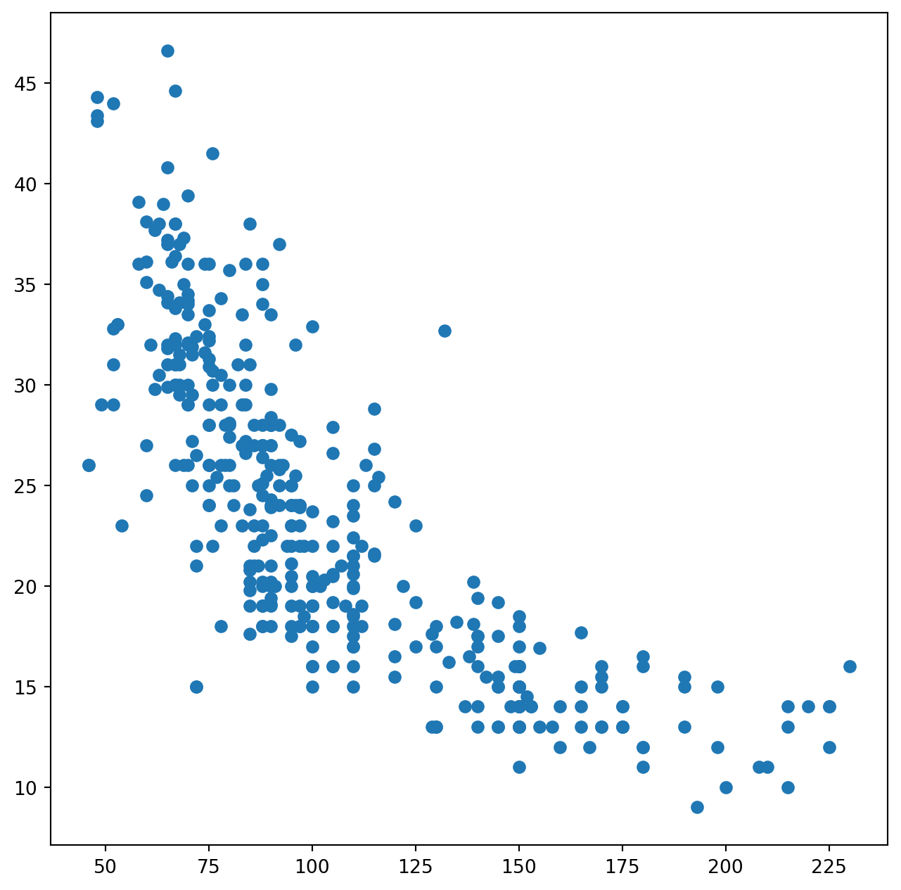

Alternatively, we can use the plot() method with the call Auto.plot(). Using this method, the variables can be accessed by name. The plot methods of a data frame return a familiar object: an axes. We can use it to update the plot as we did previously:

ax = Auto.plot.scatter('horsepower', 'mpg')
ax.set_title('Horsepower vs. MPG');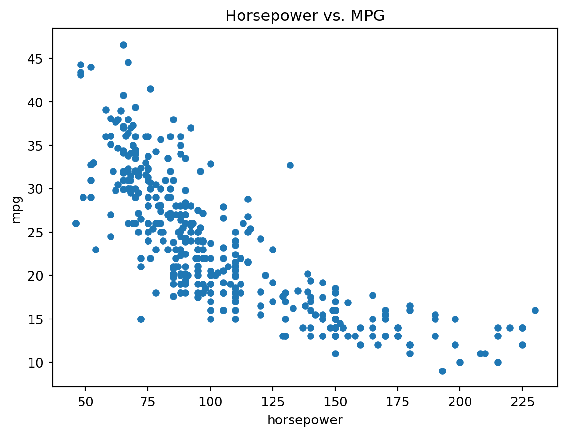

If we want to save the figure that contains a given axes, we can find the relevant figure by accessing the figure attribute:

fig = ax.figure
fig.savefig('horsepower_mpg.png');

We can further instruct the data frame to plot to a particular axes object. In this case the corresponding plot() method will return the modified axes we passed in as an argument. Note that when we request a one-dimensional grid of plots, the object axes is similarly one-dimensional. We place our scatter plot in the middle plot of a row of three plots within a figure.

fig, axes = subplots(ncols=3, figsize=(15, 5))
Auto.plot.scatter('horsepower', 'mpg', ax=axes[1]);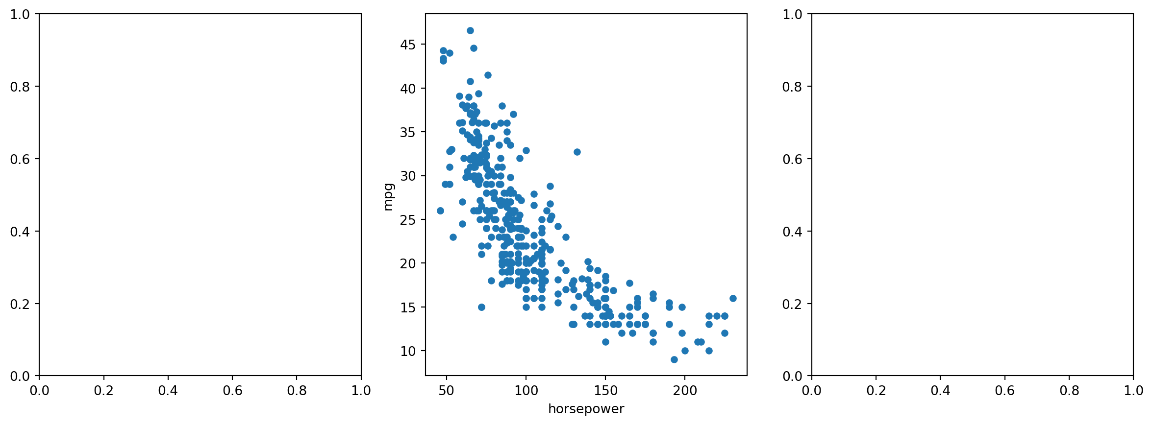

Note also that the columns of a data frame can be accessed as attributes: try typing in Auto.horsepower.

We now consider the cylinders variable. Typing in Auto.cylinders.dtype reveals that it is being treated as a quantitative variable. However, since there is only a small number of possible values for this variable, we may wish to treat it as qualitative. Below, we replace the cylinders column with a categorical version of Auto.cylinders. The function pd.Series() owes its name to the fact that pandas is often used in time series applications.

Auto.cylinders = pd.Series(Auto.cylinders, dtype='category')
Auto.cylinders.dtype

CategoricalDtype(categories=[3, 4, 5, 6, 8], ordered=False, categories_dtype=int64)

Now that cylinders is qualitative, we can display it using the boxplot() method.

fig, ax = subplots(figsize=(8, 8))
Auto.boxplot('mpg', by='cylinders', ax=ax);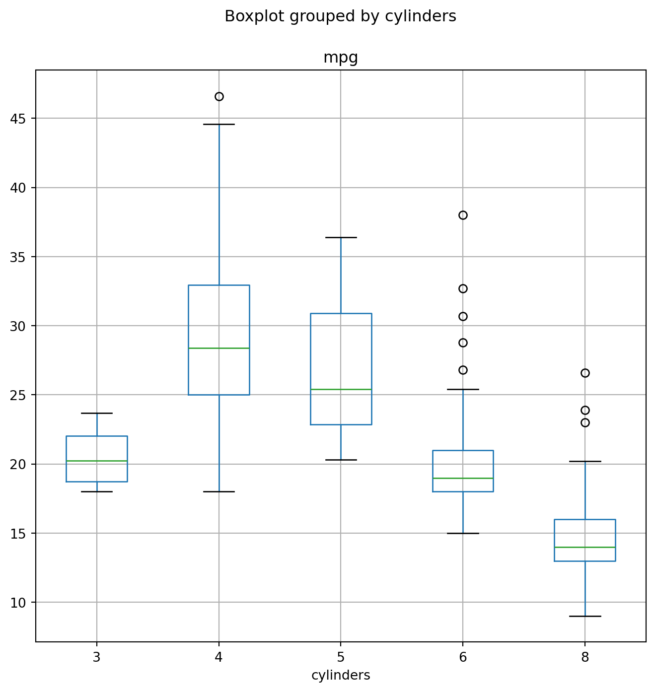

The hist() method can be used to plot a histogram.

fig, ax = subplots(figsize=(8, 8))
Auto.hist('mpg', ax=ax);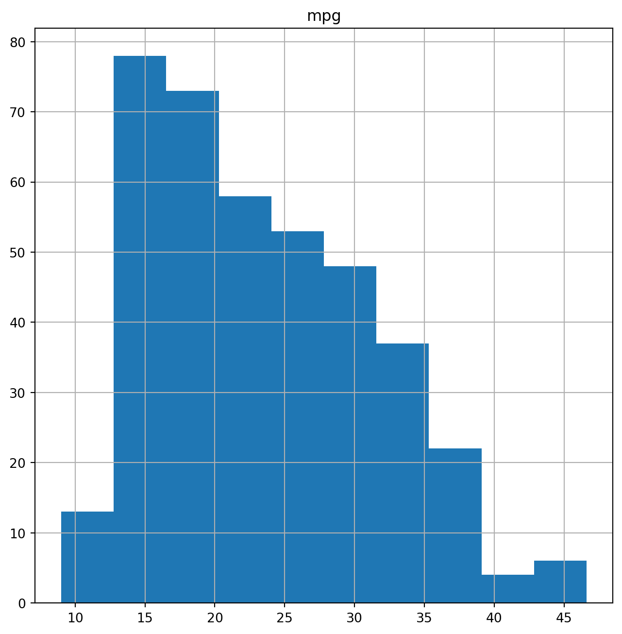

The color of the bars and the number of bins can be changed:

fig, ax = subplots(figsize=(8, 8))
Auto.hist('mpg', color='red', bins=12, ax=ax);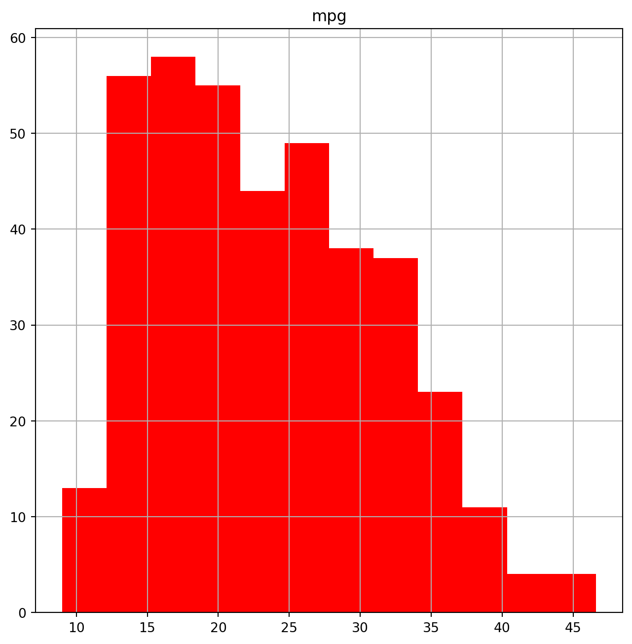

See Auto.hist? for more plotting options.

We can use the pd.plotting.scatter_matrix() function to create a scatterplot matrix to visualize all of the pairwise relationships between the columns in a data frame.

pd.plotting.scatter_matrix(Auto);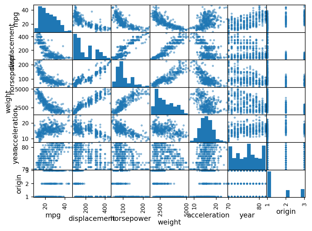

We can also produce scatterplots for a subset of the variables.

pd.plotting.scatter_matrix(Auto[['mpg',
                                 'displacement',
                                 'weight']]);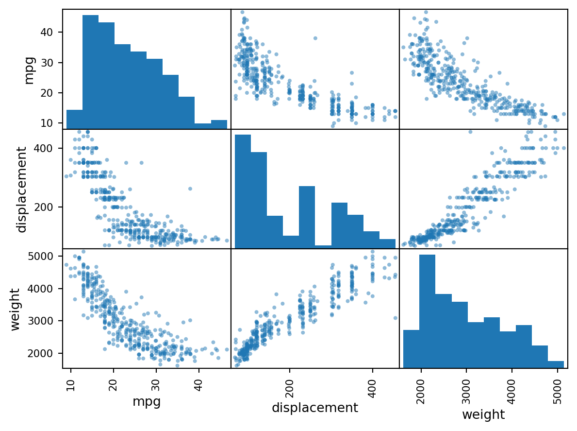

The describe() method produces a numerical summary of each column in a data frame.

Auto[['mpg', 'weight']].describe()

	mpg	weight
count	392.000000	392.000000
mean	23.445918	2977.584184
std	7.805007	849.402560
min	9.000000	1613.000000
25%	17.000000	2225.250000
50%	22.750000	2803.500000
75%	29.000000	3614.750000
max	46.600000	5140.000000

We can also produce a summary of just a single column.

Auto['cylinders'].describe()
Auto['mpg'].describe()

count     392
unique      5
top         4
freq      199
Name: cylinders, dtype: int64

count    392.000000
mean      23.445918
std        7.805007
min        9.000000
25%       17.000000
50%       22.750000
75%       29.000000
max       46.600000
Name: mpg, dtype: float64

To exit Jupyter, select File / Shut Down.