Entities should not be multiplied without necessity. – William of Ockham
The chapter is 60 pages long and covers the following topics:
- Linear Model Selection and Regularization
- Subset Selection
- Best Subset Selection
- Stepwise Selection
- Choosing the Optimal Model
- Shrinkage Methods
- Ridge Regression
- The Lasso
- Selecting the Tuning Parameter
- Dimension Reduction Methods
- Principal Components Regression
- Partial Least Squares
- Considerations in High Dimensions
- High-Dimensional Data
- What Goes Wrong in High Dimensions?
- Regression in High Dimensions
- Interpreting Results in High Dimensions
- Lab: Linear Models and Regularization Methods
- Subset Selection Methods
- Ridge Regression and the Lasso
- PCR and PLS Regression
- Exercises
- Subset Selection
There is lots of material in this chapter. Looking over it all I have a couple of pointers that seem to be outside of the scope of the book.
Model Selection makes more sense to me when we are in a Bayesian setting c.f. (Goodman, Tenenbaum, and Contributors 2016) where the authors explain about the bayesian occam’s razor. The more complex the model, the more data we need to fit it. In a Bayesian setting, we can use the posterior predictive distribution to evaluate how well a model fits the data. This is not covered in this chapter.
The authors treat Shrinkage is a way to regularize the model. This is a way to reduce the variance of the model. However there are some additional facets or benefits to shrinkage. In hierarchical models, shrinkage is a way to borrow strength from the data and we can also use prior distributions to shrink the model. Priors and the ability to transfer probability mass from known to unknown parameters in a hierarchical model can become a form of transfer learning. As we develop insights into the data generating process, we may wish to add in out subjective beliefs about its behavior. USing an inductive bias, as embodied in hierarchical models, can help us to build models that can generalize faster or give useful predictions with fewer data points. This is called few-shot learning. Finally real world data is often sparse and unbalanced. Shrinkage can help us make more educated guesses what is going on in the regions of the data we have less observation.

We cover four main topics in this chapter:
- Model selection is the process of choosing the best model from a set of candidate models. It involves evaluating trade-offs between model complexity (number of predictors) and model fit (accuracy).
- Shrinkage Methods are techniques that constrain or regularize coefficient estimates, effectively shrinking them towards zero. This helps reduce variance and improve prediction accuracy, particularly in high-dimensional datasets. Regularization techniques, such as ridge regression and lasso, help control overfitting by shrinking coefficient estimates towards zero.
- Dimension Reduction Methods like principal component regression and partial least squares, reduce the number of predictors used in a model, thus simplifying it and potentially improving performance. Understanding the bias-variance trade-off is essential for selecting the appropriate level of model complexity and regularization.
- Cross-validation is a powerful tool for selecting tuning parameters and comparing different models.
Terminology for Model Selection and Regularization
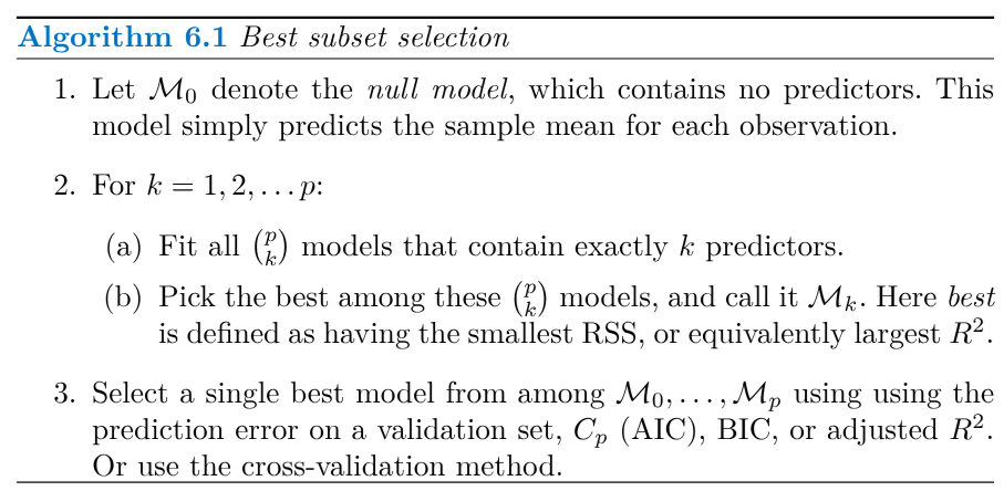
- Best Subset Selection
- A method that evaluates all possible subsets of predictor variables to find the model with the lowest training error.
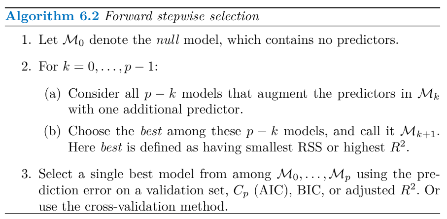
- Forward Stepwise Selection
- A method that starts with an empty model and iteratively adds the predictor that most improves the model fit at each step.
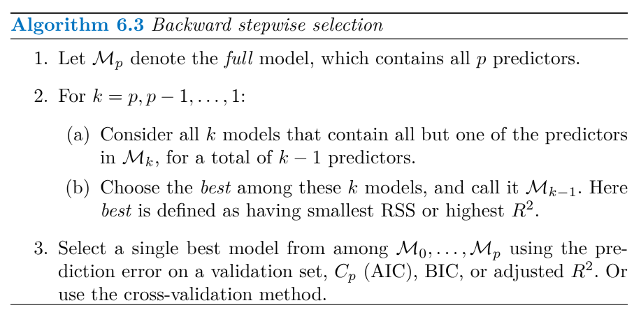
- Backward Stepwise Selection
- A method that starts with a model containing all predictors and iteratively removes the least significant predictor at each step.
- Mallow’s Cp
- A statistic used to assess the fit of a model, taking into account both the residual sum of squares and the number of parameters.
- Akaike Information Criterion (AIC)
- A metric that estimates prediction error and balances model complexity with goodness of fit, favoring simpler models.
- Bayesian Information Criterion (BIC)
- A similar metric to AIC but with a stronger penalty for model complexity, leading to even simpler models.
- Ridge Regression
- A shrinkage method that adds an L2 penalty to the least squares objective function, shrinking coefficients towards zero and reducing variance.
- Lasso
- A shrinkage method that uses an L1 penalty, forcing some coefficients to become exactly zero, leading to variable selection.
- Tuning Parameter (λ)
- A parameter that controls the strength of the penalty in shrinkage methods, balancing model fit with coefficient shrinkage.
- Cross-Validation
- A resampling technique used to estimate the performance of a model on unseen data and to select tuning parameters.
- Principal Component Regression (PCR)
- A dimension reduction technique that uses principal components (linear combinations of predictors capturing maximum variance) as predictors in regression.
- Partial Least Squares (PLS)
- A dimension reduction method that constructs components that maximize the covariance between the predictors and the response, aiming for better prediction performance.
- Multicollinearity
- A situation where predictor variables are highly correlated, which can lead to unstable coefficient estimates in least squares regression.
- Bias-Variance Trade-off
- The fundamental trade-off between model complexity and prediction accuracy. Simpler models have higher bias but lower variance, while complex models have lower bias but higher variance.
- Sparsity
- A property of a model where many of the coefficient estimates are exactly zero, indicating that only a subset of the predictors is used in the model.
- L1 Norm
- The sum of the absolute values of the elements of a vector.
- L2 Norm
- The square root of the sum of squared elements of a vector.
Outline of Chapter 6
Important Concepts:
Subset Selection Methods:
- Best Subset Selection: Evaluates all possible combinations of predictors, choosing the model with the lowest RSS (residual sum of squares) or highest R-squared. Computationally expensive for large datasets.
- Forward Stepwise Selection: Starts with a null model and iteratively adds the predictor that most improves the model fit. Continues until all predictors are included or a stopping criterion is met.
- Backward Stepwise Selection: Starts with the full model and iteratively removes the least useful predictor. Continues until a stopping criterion is met.
- Challenges: Selecting the optimal model size requires metrics that estimate test error.
- Common Metrics:
- Mallow’s C_p: Estimates test MSE (mean squared error) based on training RSS and model complexity. Seeks models with low Cp.
“Mallow’s Cp is sometimes defined as C'_p = RSS/\hat{\sigma}^2 + 2d - n. This is equivalent to the definition given above in the sense that Cp = \frac{1}{n} \hat{\sigma}^2 (C'_p + n), and so the model with smallest C_p also has smallest C'_p.”
- AIC (Akaike Information Criterion): Estimates test MSE using maximum likelihood and model complexity. Favors models with low AIC.
“The AIC criterion is defined for a large class of models fit by maximum likelihood: AIC = −2 logL+ 2 · d where L is the maximized value of the likelihood function for the estimated model.”
BIC (Bayesian Information Criterion): Similar to AIC but penalizes model complexity more heavily. Prefers simpler models with low BIC.
Adjusted R-squared: Accounts for the number of predictors in the model. Higher adjusted R-squared indicates better fit.
- Cross-Validation: Directly estimates test error by splitting data into training and validation sets.
“This procedure has an advantage relative to AIC, BIC, Cp, and adjusted R2, in that it provides a direct estimate of the test error, and makes fewer assumptions about the true underlying model.”
Shrinkage Methods:
- Ridge Regression: Shrinks coefficient estimates towards zero by adding a penalty term proportional to the sum of squared coefficients. All predictors are included in the final model.
“Ridge regression is very similar to least squares, except that the coefficients are estimated by minimizing a slightly different quantity.”
“The penalty \lambda \sum \beta^2_j in (6.5) will shrink all of the coefficients towards zero, but it will not set any of them exactly to zero unless \lambda = \infty.”
- Lasso (Least Absolute Shrinkage and Selection Operator): Shrinks coefficients by adding a penalty term proportional to the sum of absolute coefficient values. Forces some coefficients to be exactly zero, performing variable selection.
“The lasso is a relatively recent alternative to ridge regression that overcomes this disadvantage. The lasso coefficients, \hat{\beta}^L_\lambda#, minimize the quantity…”
“As with ridge regression, the lasso shrinks the coefficient estimates towards zero. However, in the case of the lasso, the %1 penalty has the effect of forcing some of the coefficient estimates to be exactly equal to zero when the tuning parameter ! is sufficiently large.”
- Benefits: Both methods improve prediction accuracy by reducing variance, but Lasso provides more interpretable models due to variable selection.
- Challenges: Selecting the optimal tuning parameter (λ or s). Cross-validation is widely used for this purpose.
Dimension Reduction Methods:
- Principal Component Regression (PCR): Constructs new variables (principal components) as linear combinations of original predictors, capturing most of the variance. Regresses the response on a subset of these components.
“PCR identifies linear combinations, or directions, that best represent the predictors X_1, \ldots , X_p.”
- Partial Least Squares (PLS): Similar to PCR but constructs components that are also related to the response variable.
- Benefits: Reduce dimensionality, potentially leading to improved prediction accuracy and model interpretability.
- Challenges: Choosing the number of components to retain. Cross-validation can be used to determine this.
Important Considerations in High Dimensions:
Traditional methods can struggle with high-dimensional data (p > n). Regularization techniques become crucial for controlling variance and preventing overfitting. Computational efficiency is essential for handling large datasets. Key Takeaways:
Choosing the right method depends on the specific dataset and the goal of the analysis. Understanding the bias-variance trade-off is essential for selecting the appropriate level of model complexity and regularization. Cross-validation is a powerful tool for selecting tuning parameters and comparing different models. Further Research:
Explore different cross-validation strategies and their performance with various model types. Investigate the theoretical properties and limitations of different model selection and regularization methods. Apply these techniques to real-world datasets and evaluate their effectiveness in practice.
Slides and Chapter
References
Reuse
Citation
@online{bochman2024,
  author = {Bochman, Oren},
  title = {Chapter 6: {Linear} {Model} {Selection} and {Regularization}},
  date = {2024-07-20},
  url = {https://orenbochman.github.io/notes-islr/posts/ch06/},
  langid = {en}
}