Advertising Models

Optimal Advertising - Dorfman–Steiner theorem (1954)

The Dorfman–Steiner theorem or condition is a theorem due to Dorfman, Robert, and Peter O. Steiner. (1954) Optimal Advertising and Optimal Quality. American Economic Review 44, 826-36..

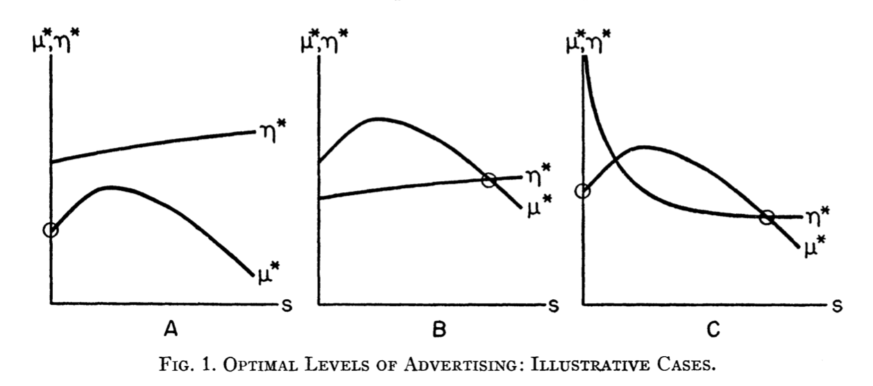
Firms can increase their sales by either decreasing the price of the good or persuading consumers to buy more by increasing advertising expenditure. The optimal level of advertising for a firm is found where the ratio of advertising to sales equals the price-cost margin times the advertising elasticity of demand.

\frac{ \text{advertising} }{ \text{sales}} = \text{price cost margin} \cdot \text{advertising elasticity of demand}

\frac{p_A A}{p \cdot q} = \frac{p-c}{p} \cdot e_A

• where:
  • p_{A} is the price per unit of advertising
  • {A} is the amount of advertising
  • p is the price of the good
  • q is the output of the good
  • c is the average or marginal cost of production
  • e_{A} is the advertising elasticity of demand.

The author of Hegji, C. E. (1998) points out that while the rule above seems intuitive, it is often misunderstood. The price in equation is taken as a fixed value for determining the marginal revenue of advertising, but Waterson (1984) stresses that both the price and level of advertising should be chosen simultaneously by the firm.

Neglecting this interaction between price and advertising is misleading and reduces the examples of using the DS rule in most textbooks to relatively simple and uninteresting ones.

The original paper also looks at more complex situation where the firm can vary both price and quality. However the authors point out that the model may be more useful for understanding the tradeoff between price and advertising rather than as a tool for making predictions. Changing price and quality and advertising are also what the game theoretic formulation of competition look at.

Wolfe Vidale sales-advertising response model (1957)

This is an early paper from the paper seems to come from the area of operations research (AKA optimization) which studies how sales responds to advertising. It tries to explains the relationship using an ODE with three parameters that allow to vary the form of the response. The authors explain that operation research (optimization techniques) may not have been applied since experimental data was hard to arrive by. They list three questions they may be able to answer using operations research:

1. Evaluating effectiveness of a campaign.
2. Budget allocation of among product and media.
3. Criteria that determine the size of the advertising budget. To formulate their ideas - they got firms to not only share data but also let them run controlled experiments in which different levels of intensity was used for advertising. According to (Wolfe and Vidale 1957) The increase in the rate os Sales is proportional to the Advertising effort reaching the fraction of available customers less the number of customers being lost. Which can be written as a first order ODE:

\frac{dS}{dt} = r A(t) \frac{M-S}{M}-\lambda S

• where:
  • S is the sales rate at time t
  • A(t) is the advertising expenditure at time t
  • \lambda is the exponential sales decay constant - which is controls the drop in sales once advertising stops. (This makes sense as people forget/remember exponentially.)
  • r is the response to advertising
  • M is the saturation level parameter (Total market size)

Developed by M.Vidal and H.Wolf. this classical advertising response model explains the rate of change of sales when advertising had both immediate and lagged effects: In this model change of the goods sales volume at time t is the function of four factors:

1. Advertising expenses
2. Constants expressing sales
3. Reaction to advertising
4. Market saturation levels with the advertised goods and constants expressing the reduction of sales volume. The basic equation of the model (advertising budget according to Vidal-Wolf formula) is :

R_b = \frac{(\Delta S + k_2 · S_0)}{ k_1} \cdot \frac{S_{max}}{(S_{max} - S_0)}

• where:
  • R_b is the advertising budget volume
  • \delta S is the change of sales volume level in comparison with the current one;
  • k_1 is the reaction constant of advertising turnover
  • S_{max} is the market saturation level of the good (job, service)
  • S_0 is the current sales volume
  • k_2 is the constant of the reduction of sales volume in the absence of advertising expenses

\frac{dS}{dt} = r \cdot A(t)\frac{(M-S)}{M} - \lambda \cdot S

• where:
  • S is the sales volume
  • A is the advertising effort
  • r is the ad effectiveness parameter
  • \lambda is the sales decay parameter
  • M is the total market size

During an advertising campaign of duration T during which spending effort is constant, sales increase, showing a concave response. When advertising ceases sales decline gradually, at a different rate than they increased.

The authors approach is to integrate which allows them to derive a number of results

A number of takeaways from this work are:

1. If a campaign has reached its saturation point continuing or discontinuing will likely to do little to improve sales. So the smart move would be to discontinuing it and put the budget else where.
2. Using pulses