116.1 Model-based state estimation
116.1.1 What are some key Kalman-filter concepts?
- KFs use sensed measurements and a mathematical model of a dynamic system to estimate its internal hidden state
- A model of the system and its state dynamics is assumed to be known.
- A system’s state is a vector of values that completely summarizes the effects of the past on the system
- The model’s state should be a twin of the system’s state
A system state vector might include the
\vec{state} =[ x,y,z, \alpha,\beta,\gamma, x', y', z', \alpha',\beta',\gamma' ] \tag{116.1}
- where:
- x, y, z are the position coordinates,
- \alpha, \beta, \gamma are the Euler angles representing the orientation of the aircraft, Or more accurately the Tait–Bryan angles
- \alpha is the roll angle,
- \beta is the pitch angle,
- \gamma is the yaw angle,
- x', y', z' are the velocities in the respective directions.
- \alpha', \beta', \gamma' are the angular velocities in the respective directions.
The number of elements in the state vector is called the state dimension or degrees of freedom.
116.1.2 Why do we need a model?
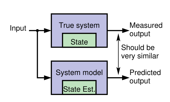
- Generally it is neither possible nor practical to measure the state of a dynamic system directly.
- According to Laplace’s view of classical mechanics if we measure the system’s inputs we can propagate those measurements through a model, updating the model’s prediction of the true state.
- We make measurements that are linear or nonlinear functions of members of the state.
- The measured and predicted outputs are compared.
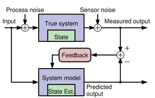
- The KF is an algorithm that updates the model’s state estimate using this prediction error as feedback regarding the quality of the present state estimate.
116.1.3 What kind of model do we assume?
Linear KFs use discrete-time state-space models of the form: \begin{aligned} x_{t+1} &= Ax_t + Bu_t + w_t && \text{state eqn.}\\ z_t &= Cx_t + Du_t + v_t && \text{observation eqn.} \end{aligned} \tag{116.2}
where:
- x_t is the state vector at time t,
- u_t is the input vector at time t,
- z_t is the output vector at time t,
- A \in \mathbb{R}^{n \times n} is the system matrix,
- B \in \mathbb{R}^{n \times r} is the input matrix,
- C \in \mathbb{R}^{m \times n} is the output matrix,
- D \in \mathbb{R}^{m \times r} is the feedforward matrix,
- w_t \sim \mathcal{N}(0,Q) is the process noise
- v_t \sim \mathcal{N}(0,R) is the sensor noise
- the state equation describes how the state evolves over time,
- the observation equation describes how the state is observed through measurements.
That too many new definitions, I feel like my hair is on fire, so here is an annotated version of the Kalman Equations: \begin{array}{rccccccl} \overbrace{x_{t+1}}^{\text{predicted state}} &= \underbrace{A}_{\text{system}} &\overbrace{\color{red} x_t}^{\text{current state}} &+ &\underbrace{B}_{\text{input}} &\overbrace{\color{green} u_t}^{\text{current input}} &+ & \underbrace{w_t}_{\text{process noise}} \\[2ex] \underbrace{z_t}_{\text{predicted output}} &= \underbrace{C}_{\text{output}} &{\color{red} x_t} &+ & \underbrace{D}_{\text{feed forward}} &{\color{green} u_t} &+ & \underbrace{v_t}_{\text{sensor noise}} \end{array} \tag{116.3}
In the NDLM we see simplified versions of these equations, where B and D are set to zero and we don’t have a current input u_t.
Another major difference explained in (Petris, Petrone, and Campagnoli 2009) is that in a statistics settings the modeler typically knows much less about the system dynamics than users of a Kalman filter who has access to some set of differential equations that describe the system dynamics.
In (West and Harrison 2013) the authors make a big point about their models being able to handle interventions.
My initial impression was that there seems to be a gap in their logic regarding this and as far as I can with the absence of the input term u(t) which should embody an interventions, these are supposed to be reflected via a change in the matrix \mathbf{F}_t,\mathbf{G}_t. However if these matrices are change every time step t, we don’t really have a model in any useful sense. (We need to somehow come up with a different model for each time step. This is not feasible even if we have access to the differential equations that describe the system dynamics.)
Looking deeper into the literature, I found that this kind of intervention is considered
in (West and Harrison 2013 ch. 11). In fact there is a whole chapter dedicated to interventions and monitoring where the authors eventually discuss arbitrary interventions.
It appears that the interventions seem to lead to the same form being used but with either an additional term for the noise or an expansion of G to incorporate an expansion of the state vector to include new parameters that if such are required.
(Prado, Ferreira, and West 2023, 154) also discusses three types of interventions but not in the same depth as the above.
- Treating y_t as an outlier
- Increasing uncertainty at the system level by adding a second error term to the state equation.
- Arbitrary intervention by setting the prior moments of the state vector to some specific values.
\begin{array}{rccccl} \overbrace{x_{t+1}}^{\text{predicted state}} &= \underbrace{G}_{\text{system}} &\overbrace{\color{red} x_t}^{\text{current state}} &+ & \underbrace{w_t}_{\text{process noise}} \\ \underbrace{y_t}_{\text{predicted output}} &= \underbrace{F}_{\text{output}} &{\color{red} x_t} &+ & \underbrace{v_t}_{\text{sensor noise}} \end{array} \tag{116.4}
116.1.4 A simple example model
Concrete example: Consider the 1-d motion of a rigid object.
- The state comprises position p_t and velocity (speed) s_t : \underbrace{\begin{bmatrix} p_t \\ s_t \end{bmatrix}}_{x_t} = \underbrace{\begin{bmatrix} 1 & \Delta t \\ 0 & 1 \end{bmatrix}}_{A} \underbrace{\begin{bmatrix} p_{k-1} \\ s_{k-1} \end{bmatrix}}_{x_{k-1}} + \underbrace{\begin{bmatrix} 0 \\ \Delta t \end{bmatrix} }_{B} u_{k-1} + w_{k-1} \tag{116.5}
- where \Delta t is the time interval between iterations t-1 and t .
- u_t is equal to force divided by mass;
- w_t is a vector that perturbs both p_t and s_t .
The measurement could be a noisy position estimate: z_t = \underbrace{\begin{bmatrix} 1 & 0 \end{bmatrix}}_{C} \underbrace{\begin{bmatrix} p_t \\ s_t \end{bmatrix}}_{x_t} + v_t \tag{116.6}
Example illustrates how the state-space form can model a specific dynamic system.
The form is extremely flexible: can be applied to any finite-dimensional linear system.
116.1.5 Why do we need feedback?
Our goal is to make an optimal estimate of x_t in: Equation 116.2
If we knew x_0, w_t, and v_t perfectly, and if our model were exact, there would be no need for feedback to estimate x_t at any point in time. We simply simulate the model! However, in practice:
- We rarely know the initial conditions x_0 exactly
- We never know the system or measurement noise w_t, v_t (by definition).
- Also, no physical system is truly linear and even if one were, we would never know A, B, C, and D exactly.
So, simulating the model (specifically, simulating the state equation “open loop”) is insufficient for robust estimation of x_t.
- Feedback allows us to compare predicted z_t with measured z_t to adjust x_t.
116.1.6 How does the feedback work?
- Discrete-time Kalman filters repeatedly execute two steps:
- Predict the current state-vector values based on all past available data. E.g., a linear KF computes \hat{x}_t^- = A \hat{x}_{t-1}^+ + B u_{t-1} \tag{116.7}
- where
- \hat{x}_{t-1}^+ is the prediction of x_{t-1}.
- \hat{x}_{t-1}^- is the estimate of x_{t-1}.
- Estimate the current state value by updating the prediction based on all presently available data. E.g., a linear KF computes \hat{x}_{t}^+ = \hat{x}_t^- + {\textcolor{blue} {L_t}}\, (z_t - (C \hat{x}_t^- + D u_t)) \tag{116.8}
- A very straightforward idea. But …
- What should be the feedback gain matrix L_t?
- That is, how do we make this feedback optimal in some meaningful sense?
- What should be the feedback gain matrix L_t?
- Can we generalize this feedback concept to nonlinear systems?
- What if we don’t know u_t (as in the tracking application)?
116.1.7 Summary
- KFs use sensed measurements and a mathematical model of a dynamic system to estimate its internal hidden state.
For the kind of KFs we will study, the mathematical model must be formulated in a discrete-time state-space format.
This form is very general, and can apply to nearly any dynamic system of interest.
KFs operate by repeatedly predicting the present state, and then updating that prediction using a measured system output to make an estimate of the state.
This process is optimized by computing an optimal feedback gain matrix L_t at every time step that blends the prediction and the new information in the measurement.
There is a lot to learn, and the next topic will present our roadmap for doing so.
116.2 Working through a KF example at high-level
116.2.1 A problem for which KF should be a good solution
- We will now walk through an example—without going into all the details—to illustrate how a KF works.
- Consider a car traveling in a straight line. We would like to estimate its position.
- We use GPS as a position sensor—but GPS estimates have measurement uncertainty and we wonder if blending our knowledge of the car’s dynamics with GPS might let us infer a better position estimate.
- We might think, “Maybe we could use a Kalman filter to estimate the car’s position better than simply using GPS.”
- We would be right!
116.2.2 Designing the Kalman filter: The model
- To design the KF, we require a discrete-time state-space model of the dynamics of the car.
- We adopt the model of 1-d motion of a rigid object from the prior lesson.
- The state comprises position pk and velocity (speed) s_t :
\begin{bmatrix} p_t \\ s_t \end{bmatrix} = \begin{bmatrix} 1 & \Delta t \\ 0 & 1 \end{bmatrix} \begin{bmatrix} p_{k-1} \\ s_{k-1} \end{bmatrix} + \begin{bmatrix} 0 \\ \Delta t \end{bmatrix} u_{k-1} + w_{k-1}
where \Delta t is the time interval between iterations t-1 and t . - u_t is equal to force divided by mass; - w_t is a vector that perturbs both p_t and $s
The measurement is a noisy GPS position estimate: z_t = \begin{bmatrix} 1 & 0 \end{bmatrix} \begin{bmatrix} p_t \\ s_t \end{bmatrix} + v_t
116.2.3 Designing the Kalman filter: The uncertainties
- We also need to describe what we know about the uncertainties of the scenario.
- What do we know about the initial state of the car, x_0 ?
- What do we know about process noise w_t (wind) affecting the state’s evolution?
- What do we know about the measurement noise v_t (GPS measurement error)?
- For most of the specialization, we will assume that these uncertainties are described by Gaussian (normal) distributions, which can be specified if we know the means and standard deviations of the probability density functions. We assume:
- That GPS measurement error has zero mean and standard deviation of 1.5 m. The overall confidence is then about 4.5 m.
- That x_0 is initialized via a GPS measurement, so has zero mean and standard deviation of 5 ft.
- That w_t has zero mean and a standard deviation of 3cm\; s^{-1} on the velocity state.
116.2.4 Visualizing the Kalman-filter process: Prediction
- We first initialize the KF state estimate for iteration t = 0. x_0 is uncertain since it is estimated from a GPS measurement.
- We draw this uncertainty as a shaded blue pdf.
- We don’t know the car’s position exactly; but we do know where we expect it to be (at the measurement location) and we know the range of likely true locations (about \pm 4.5 m).
- One time-step later, the car has moved.
- The KF uses the model plus knowledge of u_t to predict where the car will be, drawn as the shaded yellow pdf.
- Since we do not know w_t, the uncertainty of the position estimate has increased.
116.2.5 Visualizing the Kalman-filter process: Estimation
- At this point, we make a GPS measurement of the car’s new position, remembering that the measurement has uncertainty.
- Again, we show this as a shaded blue pdf.
- We now have an uncertain prediction of the position from the model (yellow) and an uncertain measurement (blue).
- We need to combine these.
- The KF takes into consideration the prediction and the measurement and their uncertainties to compute an estimate of the car’s location.
- This estimate (green) will be optimal in some sense, and will have less uncertainty than either the prediction or the measurement.
116.2.6 Properties of the Kalman-filter solution
The KF repeatedly takes two steps: prediction and correction.
- The prediction step uses the known dynamics of the state and known characteristics of the process noise w_t.
- The correction step combines the prediction and the measurement and their uncertainties to make a state estimate valid for this time step.
The output of the KF at every time step comprises two quantities: the state estimate and confidence bounds on this estimate.
The KF never “knows” the true system state exactly and does not converge to the true state (i.e., with vanishingly small confidence bounds) over time, since process noise w_t continuously modifies the state in unknown ways.
But, the confidence bounds allow us to interpret the output of the KF appropriately.
116.2.7 Summary
- This lesson has illustrated KF operation for a specific example.
- We learned that we will need to specify a model of the system and the uncertainties of the signals in the model.
- We will need to initialize the KF with an estimate of x_0.
- Then, every measurement interval we perform a prediction and a correction step.
- Prediction increases uncertainty and correction decreases uncertainty. The KF “fuses” the prediction with the measurement to make an optimal estimate.
- The output of the KF is the state estimate as well as its confidence bounds.
- The estimate will always contain some randomness due to w_t, so the confidence bounds will not decay to zero width.
- The confidence bounds are necessary so we know the estimate’s accuracy level.
116.3 What is a state-space model and why do I need to know about them?
116.3.1 Example of a continuous-time state-space model
Representation of the dynamics of an nth-order system as a first-order differential equation in an n-vector called the state
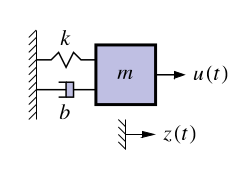
Classic example: Second-order equation of motion
\begin{aligned} m\ddot{z}(t) &= u(t) - b \dot{z}(t) -k z(t) \\ \ddot{z}(t) &= \frac{1}{m} u(t) - \frac{b}{m} \dot{z}(t) -\frac{k}{m} z(t) \\ \end{aligned} \tag{116.9}
- where:
- z(t) is the position of the mass at time t,
- \dot{z}(t) is the velocity of the mass at time t,
- k is the spring constant,
- m is the mass,
- b is the damping coefficient,
- We can define a (non-unique) state vector which embodies the system’s state at time t as: \begin{aligned} x(t) &= \begin{bmatrix} z(t) \\ \dot{z}(t) \end{bmatrix} \\ \dot{x}(t) &= \begin{bmatrix} \dot{z}(t) \\ \ddot{z}(t) \end{bmatrix} &= \begin{bmatrix} \dot{z}(t) \\ \frac{1}{m} u(t) - \frac{b}{m} \dot{z}(t) -\frac{k}{m} z(t) \end{bmatrix} \end{aligned} \tag{116.10}
116.3.2 Example in continuous-time state-space form
- So far we have: \begin{aligned} \dot{x}(t) &= \begin{bmatrix} \dot{z}(t) \\ \ddot{z}(t) \end{bmatrix} &= \begin{bmatrix} \dot{z}(t) \\ \frac{1}{m} u(t) - \frac{b}{m} \dot{z}(t) -\frac{k}{m} z(t) \end{bmatrix} \end{aligned}
We can write this as \dot x(t) = Ax(t) C + Bu(t), where A and B are constant matrices
\begin{aligned} \dot{x}(t) &= \begin{bmatrix} \dot{z}(t) \\ \ddot{z}(t) \end{bmatrix} &= \underbrace{\begin{bmatrix} ? &? \\ ?& ? \end{bmatrix} }_{A} \begin{bmatrix} \dot{z}(t) \\ \ddot{z}(t) \end{bmatrix} + \underbrace{\begin{bmatrix} ? &? \\ ?& ? \end{bmatrix} }_{B} u(t) \end{aligned}
- Complete the model by computing z(t) = C x(t)+ C Du(t) , where C and D are constant matrices
C = \begin{bmatrix} ?, ?, ?, ? \end{bmatrix} \qquad D = \begin{bmatrix} ?, ? \end{bmatrix}
116.3.3 Standard state-space model form
Standard form for continuous-time linear state-space model: \begin{aligned} \dot{x}(t) &= A x(t) + B u(t) + w(t) \\ z(t) &= C x(t) + D u(t) + v(t) \end{aligned} \tag{116.11}
- where
- u(t) is the known input,
- x(t) is the state,
- A, B, C , D are constant matrices.
- where
Convenient way to express dynamics (matrix format great for computers).
The first equation is called the state equation or the process equation.
- Only this equation evolves over time (since it is a first-order vector ODE that integrates the right-hand side to find x(t) ).
- So, this equation summarizes the “dynamics” of the model.
The second equation is called the output equation or the measurement equation.
- It is a static linear combination of variables known at time t.
116.3.4 What is the system state vector?
Standard form for continuous-time linear state-space model: \begin{aligned} \dot{x}(t) &= A x(t) + B u(t) + w(t) \\ z(t) &= C x(t) + D u(t) + v(t) \end{aligned}
We think of the system state at time t_0 as a minimum set of information at t_0 that, together with input u(t), t \geq t_0, uniquely determines system behavior for all t \geq t_0.
- State variables provide access to what is going on inside the system.
- The state has dimensions x(t) \in \mathbb{R}^n, so A \in \mathbb{R}^{n \times n} and w(t) \in \mathbb{R}^n.
Note that in principle we can solve the state equation numerically, x(t) = x(0) + \int_{0}^{t} A x(\tau) + B u(\tau) + w(\tau) d\tau \tag{116.12}
However, it will usually be more convenient to keep the equation in differential form.
116.3.5 What are the output and inputs?
\begin{aligned} \dot{x}(t) &= A x(t) + B u(t) + w(t) \\ z(t) &= C x(t) + D u(t) + v(t) \end{aligned}
- The model output is z(t) \in \mathbb{R}^m. This is the measurement we make.
- There are three input signals to the model: u(t), w(t), and v(t).
- We consider u(t) \in \mathbb{R}^r to be a deterministic input that is, we assume that we know its value exactly at all times.
- Based on the size of u(t); we infer that B \in \mathbb{R}^{n \times r}.
- The deterministic input forces x(t) to evolve over time in different ways, depending on its values.
- It also influences the output via the D term.
116.3.6 What are the random (stochastic) inputs?
\begin{aligned} \dot{x}(t) &= A x(t) + B u(t) + w(t) \\ z(t) &= C x(t) + D u(t) + v(t) \end{aligned} \tag{116.13}
- The model has two random input signals: w(t), and v(t).
- They are random in the sense that we assume that we never know their values exactly.
- We have already seen that w(t) \in \mathbb{R}^n; if v(t) \in \mathbb{R}^m, then v(t) \in \mathbb{R}^m also. The w(t) signal is process noise. Notice that it affects the dynamics of the model by making direct changes to the evolution of x(t).
- The v(t) signal is sensor noise. Notice that it does not affect the dynamics of the model; it affects only the measurement z(t).
- Systems having noise inputs w(t) and v(t) are considered in detail in week 3.
116.3.7 What are the matrices called?
The standard form for linear continuous-time state-space models is \begin{aligned} \dot{x}(t) &= A x(t) + B u(t) + w(t) \\ z(t) &= C x(t) + D u(t) + v(t) \end{aligned} \tag{116.14}
A \in \mathbb{R}^{n \times n} is the system matrix. It models the evolution of the state in the absence of input.
B \in \mathbb{R}^{n \times r} is the input matrix. It defines how linear combinations of u(t) impact the evolution of the state.
C \in \mathbb{R}^{m \times n} is the output matrix. It defines how the output depends on linear combinations of states.
D \in \mathbb{R}^{m \times r} is the feed–forward (or feed–through) matrix. It models how the output depends on linear combinations of the input (instantaneously).
Time-varying systems have A, B, C, D that change with time.
116.3.8 Why do you need to know about them?
- It can be of vital interest to know the state of the system, but we usually cannot measure it directly.
- Instead, we can measure u(t) and z(t), and although we cannot measure the random signals w(t) and v(t), we can model some of their critical attributes.
- This enables us to make methods to estimate x(t) based on what we measure and what we model.
- Kalman filters are (in some cases optimal) estimators of x(t)
- The derivation and implementation of the KF depends on modeling the system in state-space form and having knowledge of the model A, B, C, and D matrices.
- This is why we care!
116.3.9 Summary
State-space models are a compact representation of an n^th^-order linear system in terms of a 1st-order vector ODE.
The standard form for linear continuous-time state-space models is Equation 116.14
We have learned the names of the equations, the names of the matrices, and the names of the signals (and what they all mean).
We have seen one example of a model in state-space form;
Next, we will look at three other important general models.