Notes from Udacity A/B Testing course, I took this course around the time it first launched. The course is about planning and analyzing A/B tests - not about implementing A/B testing using a specific framework.
Metrics Difference between click-through rate and click-through probability?
CTR is used to measure usability e.g. how easy to find the button, \(\frac{ \text { click}}{\text{ page views}}\).
CTP is used to measure the impact \(\frac{ \text {unique visitors click}}{\text{ unique visitors view the page}}\).
Statistical significance and practical significance
Statistical significance is about ensuring observed effects are not due to chance.
Practical significance depends on the industry e.g. medicine vs. internet.
Statistical significance
\(\alpha\): the probability you happen to observe the effect in your sample if \(H_0\) is true.
Small sample: \(\alpha\) low, \(\beta\) high.
Larger sample, \(\alpha\) same, \(\beta\) lower
any larger change than your practical significant boundary will have a lower \(\beta\), so it will be easier to detect the significant difference.
\(1-\beta\) also called sensitivity
How to calculate sample size?
Use this calculator, input baseline conversion rate, minimum detectable effect (the smallest effect that will be detected \((1-\beta)%\) of the time), alpha, and beta.
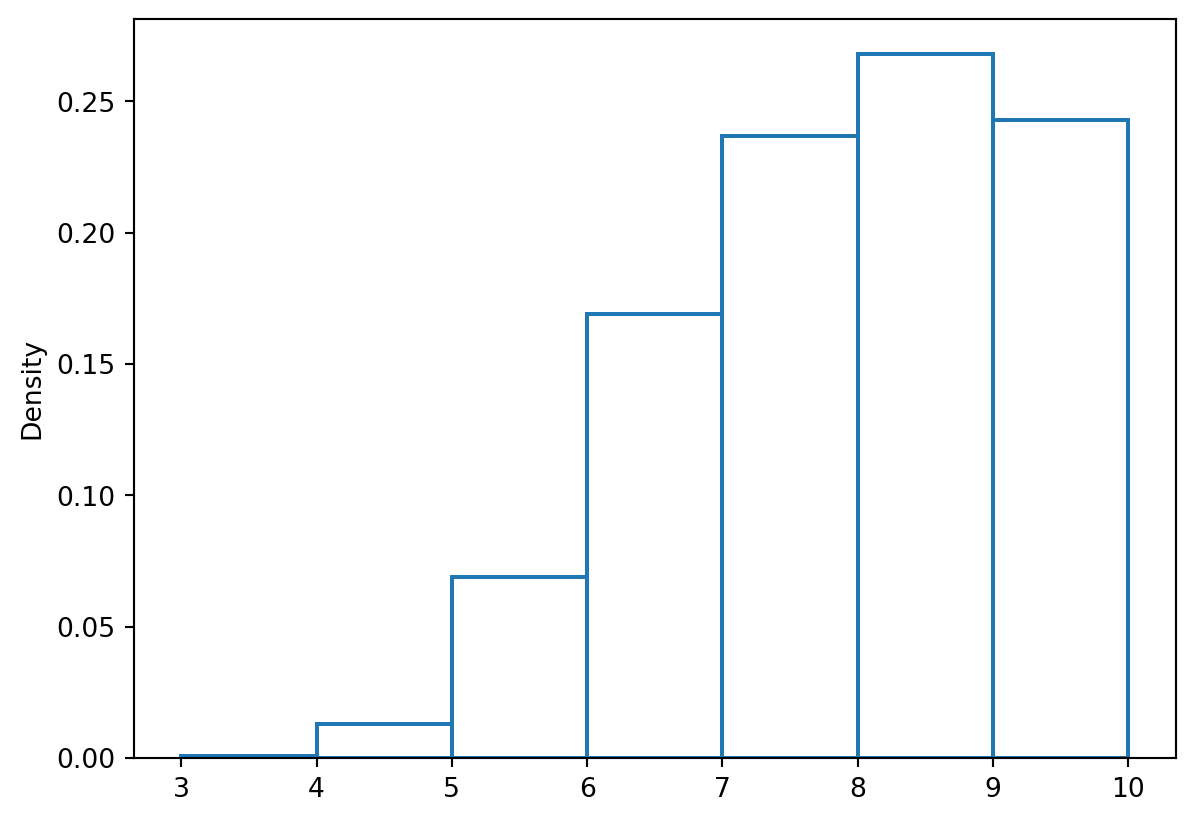
np.set_printoptions(formatter={'float':"{0:0.2f}".format})np.set_printoptions(precision=2)mean = np.round(x.mean(),2)mean_theoretical = np.round(n_trials* p,2)width=6print(f'mean {mean:<{width}} mean_theoretical {mean_theoretical}')variance = np.round(x.var(),2)variance_theoretrical = np.round(n_trials* p * (1-p),2)print(f'var {variance:<{width}} var_theoretrical {variance_theoretrical}')sd = np.round(x.std(),2)sd_theoretical = np.round(np.sqrt(variance_theoretrical),2)print(f'sd {sd:<{width}} sd_theoretical {sd_theoretical}')##TODO can we do it with PYMC, in a tab
mean 7.47   mean_theoretical  7.5
var  1.93   var_theoretrical  1.88
sd   1.39   sd_theoretical    1.37
n=n_trialsconfidence =95/100alpha=1-confidencez=1-(1/2)*alphaci=np.round(z+np.sqrt(p_est*(1-p_est)/n_trials),2)print(f'{alpha=},{z=}')print(f'[-{ci},{ci}] wald ci')z_lb=1-(1/2)*alphaz_ub=1-(1/2)*(1-alpha)print(f'{alpha=},{z_lb=},{z_ub=}')lb_wilson=(p_est+z_lb*z_lb/(2*n)+z_lb*np.sqrt(p_est*(1-p_est)/n + z_lb*z_lb/(4*n)))/(1+z_lb*z_lb/n)ub_wilson=(p_est+z_ub*z_ub/(2*n)+z_ub*np.sqrt(p_est*(1-p_est)/n + z_ub*z_ub/(4*n)))/(1+z_ub*z_ub/n)print(f'[-{lb_wilson},{ub_wilson}] wilson ci')
alpha=0.050000000000000044,z=0.975
[-1.07,1.07] wald ci
alpha=0.050000000000000044,z_lb=0.975,z_ub=0.525
[-0.2958906056936498,0.17513456528071358] wilson ci