In week 1 we define some key concepts like rewards, states, action, value functions, action values functions. We consider the the multi-armed bandit problem, leading to exploration explotation dillema, and the epsilon greedy algorithm.
Coursera
Fundamentals
Reinforcement Learning
Published
Monday, May 2, 2022
Keywords
the k-armed bandit problem, bandit algorithms, exploration, exploitation, epsilon greedy algorithm, sample average method
RL logo
RL algorithms
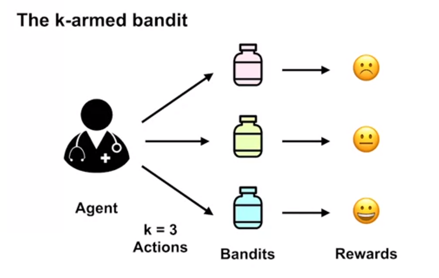
Lesson 1: The K-Armed Bandit
TipRead
NoteGoals
In reinforcement learning, the agent generates its own training data by interacting with the world. The agent must learn the consequences of his own actions through trial and error, rather than being told the correct action – (Matha White 2020)
K-armed bandits 🐙
In the k-armed bandit problem there is an agent who is assigned a states by the environment and must learn which action a from the possible set of actionsA leads to the goal state through a signal based on the greatest expected reward.
One way this can be achieved is using a Bayesian updating scheme starting from a uniform prior.
Temporal nature of the bandit problem
The bandit problem cam be static problem with a fixed reward distribution. However, more generally it is a temporal problem when the rewards distribution changes over time and agent must learn to adapt to these changes.
NoteDifference between bandits and RL
In the typical bandit setting there is only one state. So after we pull the arm nothing in the problem changes.
Bandits problems where agents can discriminate between states are called contextual bandits.
However, bandits embody one of the main themes of RL - that of estimating an expected reward for different actions.
In the more general RL setting we will be interested in more general problems where actions will lead the agent to new states and the goal is some specific state we need to reach.
\mathbb{E}[r \vert a] means expectation of a reward given some action a Since agents want to maximize rewards, recalling the definition of expectations we can write this as:
The goal of the agent is to maximize the expected reward which we can express mathematically as:
\arg\max_a q(a)=\sum_r p(r \vert a) \times r \qquad \text{(Greedification)}
\tag{2}
where:
\arg \max_a means the argument a maximizes - so the agent is looking for the action that maximizes the expected reward and the outcome is an action.
Reward, Return, and Value Functions
The rewardr is the immediate feedback from the environment after the agent takes an action.
The returnG_t is the total discounted reward from time-step t.
The value functionv(s) of an MRP is the expected return starting from state s.
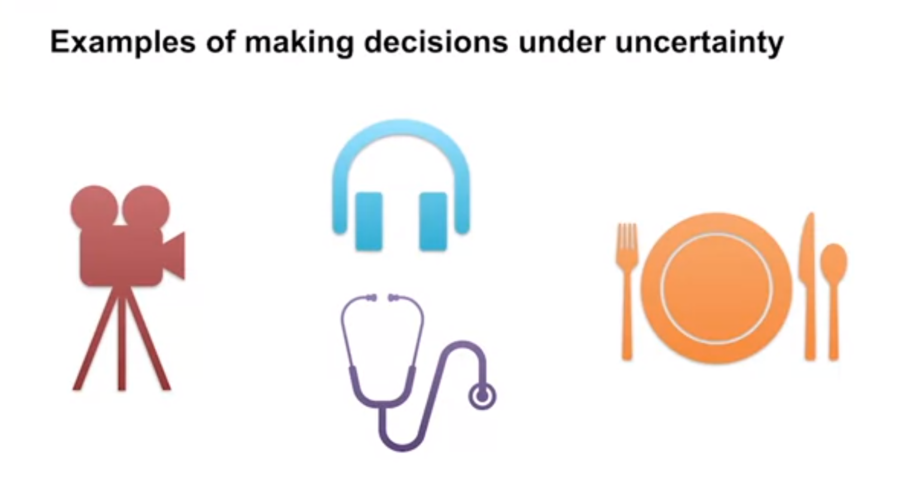
decisions
example of decisions under uncertainty:
movie recommendation.
clinical trials.
music recommendation.
food ordering at a restaurant.
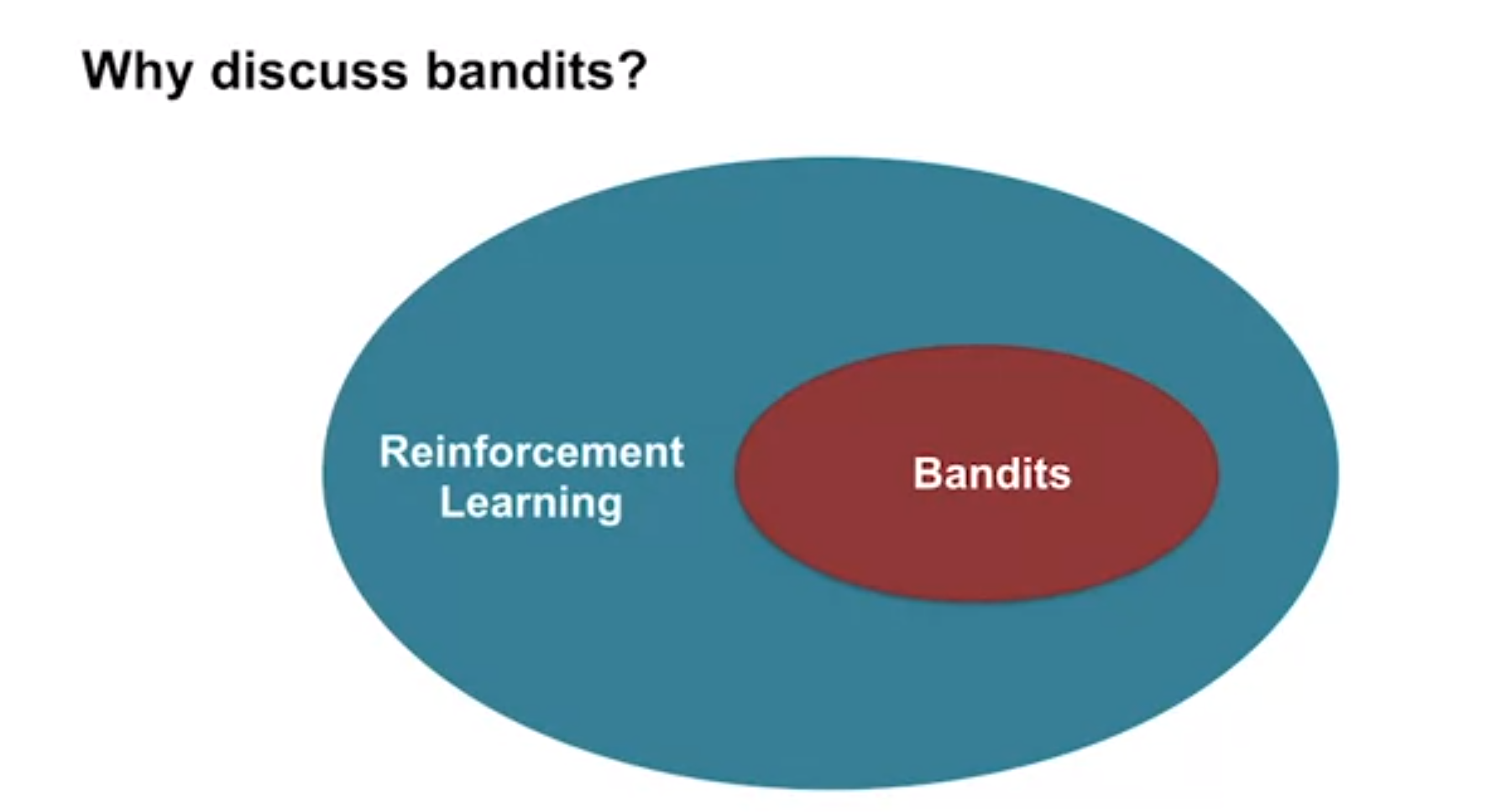
why discuss bandits
It best to consider issues and algorithms design choices in the simplest setting first. The bandit problem is the simplest setting for RL. More advanced algorithms will incorporate parts we use to solve this simple settings.
maximizing rewards.
balancing exploration and exploitation.
estimating expected rewards for different actions.
are all problems we will encounter in both the bandit and the more general RL setting.
Lesson 2: What to learn: understanding Action Values
NoteGoals
What are action-value estimation methods?
estimating action values
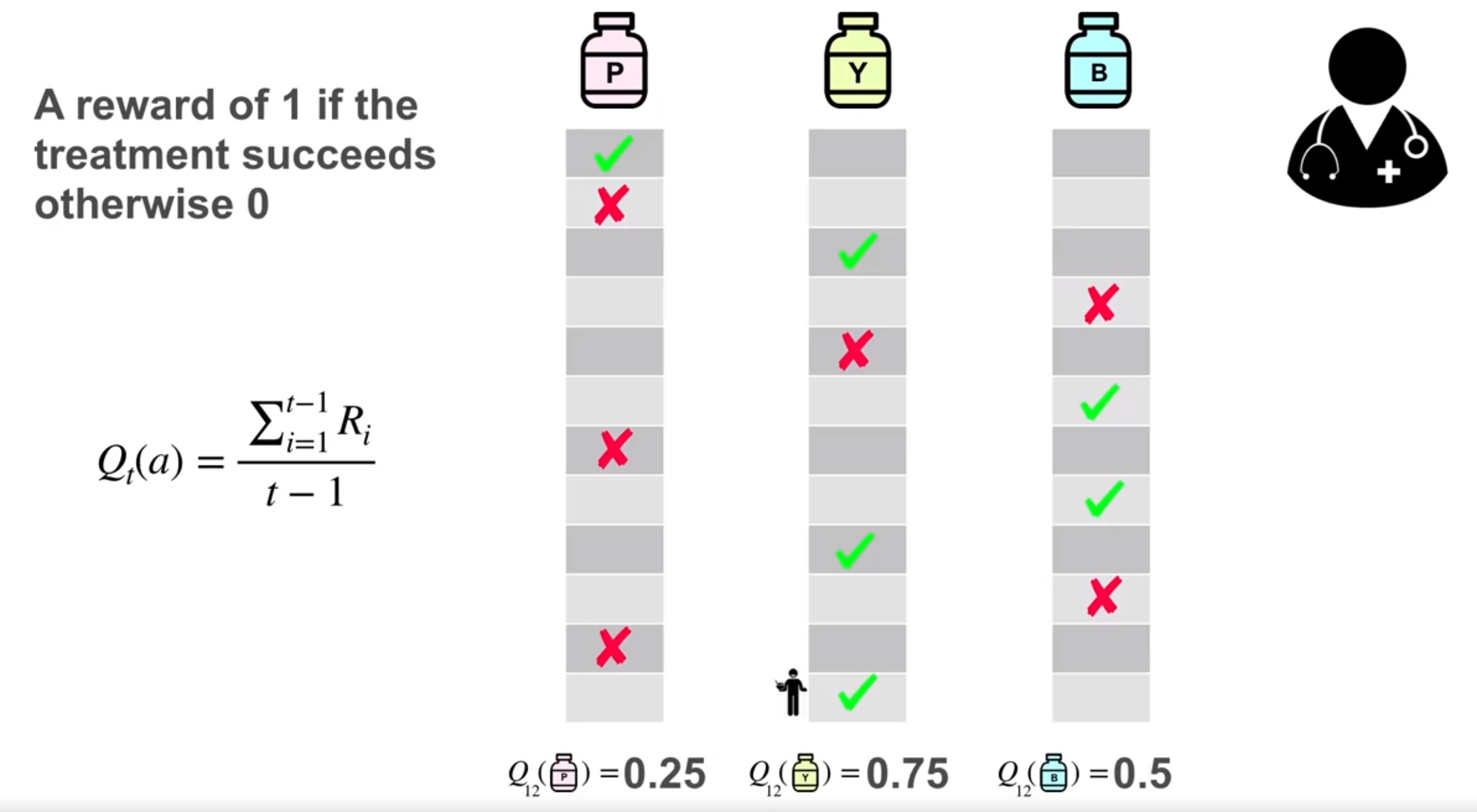
In Tabular RL settings The action value function q is nothing more than a table with one {state, action} pair per row and its value. More generally, like when we will consider function approximation in course 3, it is a mapping from {state, action} pair to a expected reward.
State s
Action a
Action value q(s,a)
0
red treatment
0.25
0
yellow treatment
0.75
0
blue treatment
0.5
The higher the action value q(a) of an action a, the more likely it is to lead us to a better state which is closer to the objective. We can choose for each state the best or one of the best choices giving us a plan for navigating the state space to the goal state.
Q_t(a) \doteq \frac{\text{sum of rewards for action a taken time } t}{\text{number of times action a was taken prior to } t} = \frac{\sum_{i=1}^{t-1} R_i}{t-1} \qquad
\tag{3}
The main idea of RL is that we can propagate values from an one adjacent state to another. We can start with the uniform stochastic policy and use it to estimate/learn the action values. Action values will decrease for actions leads to a dead end. And it will increase in the direction of the goal but only once the influence of the goal has propagated. A continuing theme in RL is trying to increase the efficiency for propagation of rewards across the action values.
Knowing the minimum number of action needed to reach a goal can be an approximate indicator of the action value.
A second idea is that once we have let the influence of dead end and the goals spread enough we may have enough information to improve the initial action value to a point where each action is the one of the best choices. We call picking the one of the best action greedy selection and it leads to a deterministic policy. This is the optimal policy, it might not be unique since some actions might be tied in terms of their rewards. However for all of these we cannot do any better.
Exploration and Exploitation definition and dilemma
In the bandit setting we can define:
Exploration
Testing any action that might be better than our best.
Exploitation
Using the best action.
Should the doctor explore new treatments that might harm his patients or exploit the current treatment. In real life bacteria gain immunity to antibiotics so there is merit to exploring new treatments. However, a new treatment can be harmful to some patients. Ideally we want to enjoy the benefits of the best treatment but to be open to new and better alternatives but we can only do one at a time.
Since exploitation is by definition mutually exclusive with exploration we must choose one and give up the benefits of the other. This is the dilemma of Exploration and Exploitation. How an agent resolves this dilemma in practice depends on the agent’s preferences and the type of state space it inhabits, if it has just started or encounters a changing landscape it should make an effort to explore, on the other hand if it has explored enough to be certain of a global maximum it would prefer to exploit.
Defining Online learning ?
Online learning
learning by updating the agent’s value function or the action value function step by step as an agent transverses the states seeking the goal. Online learning is important to handle MDP which can change.
One simple way an agent can use online learning is to try actions by random and keep track of the subsequent states. Eventually we should reach the goal state. If we repeat this many times we can estimate the expected rewards for each action.
Sample Average Method for estimating Action Values Incrementally
Action values help us make decision. Let’s try and make estimate action values more formal using the following method:
q_t(a)=\frac{\text{sum or rewards when a taken prior to t}}{\text{number of times a taken prior to t}}
=\frac{\sum_{t=1}^{t-1} R_i \mathbb{I}_{A_i=a}}{\sum_{t=1}^{t-1}\mathbb{I}_{A_i=a} } \qquad
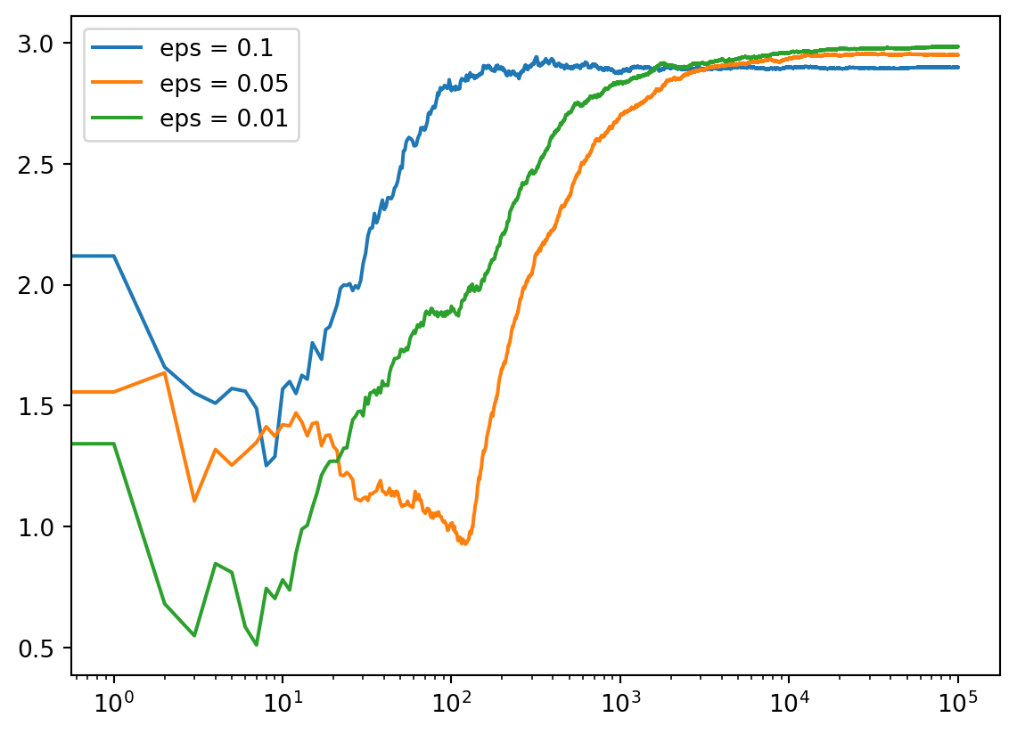
The Ɛ-greedy policy uses a simple heuristic to balance exploration with exploitation. The idea is to choose the best action with probability 1-\epsilon and to choose a random action with probability \epsilon.
A problem with Ɛ-greedy is that it is not optimal in the long run.
Even after it has found the best course of action it will continue to explore with probability \epsilon.
This is because the policy is not adaptive.
One method is too reduce \epsilon over time. However unless there is a feedback from the environment this will likely stop exploring too soon or too late thus providing sub-optimal returns.
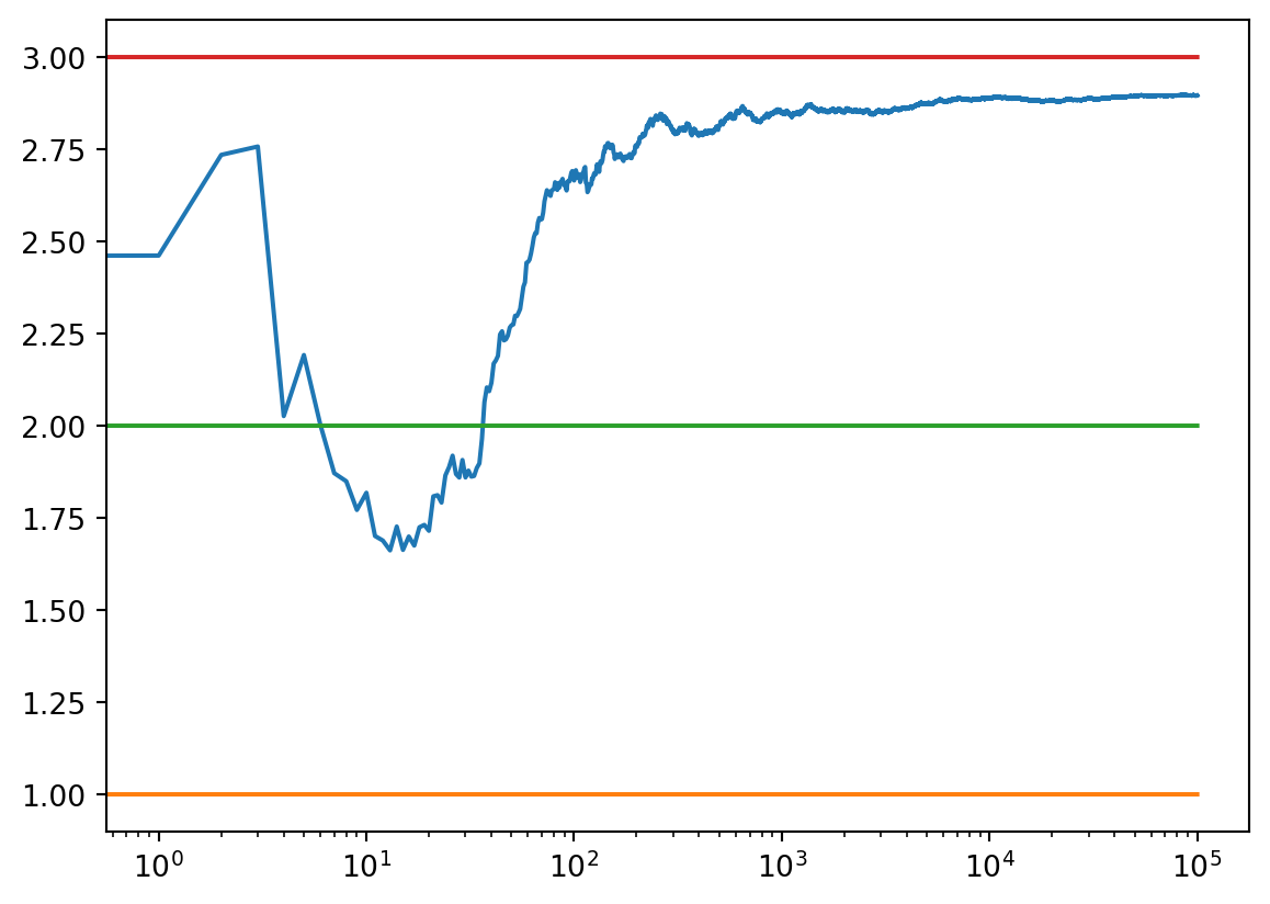
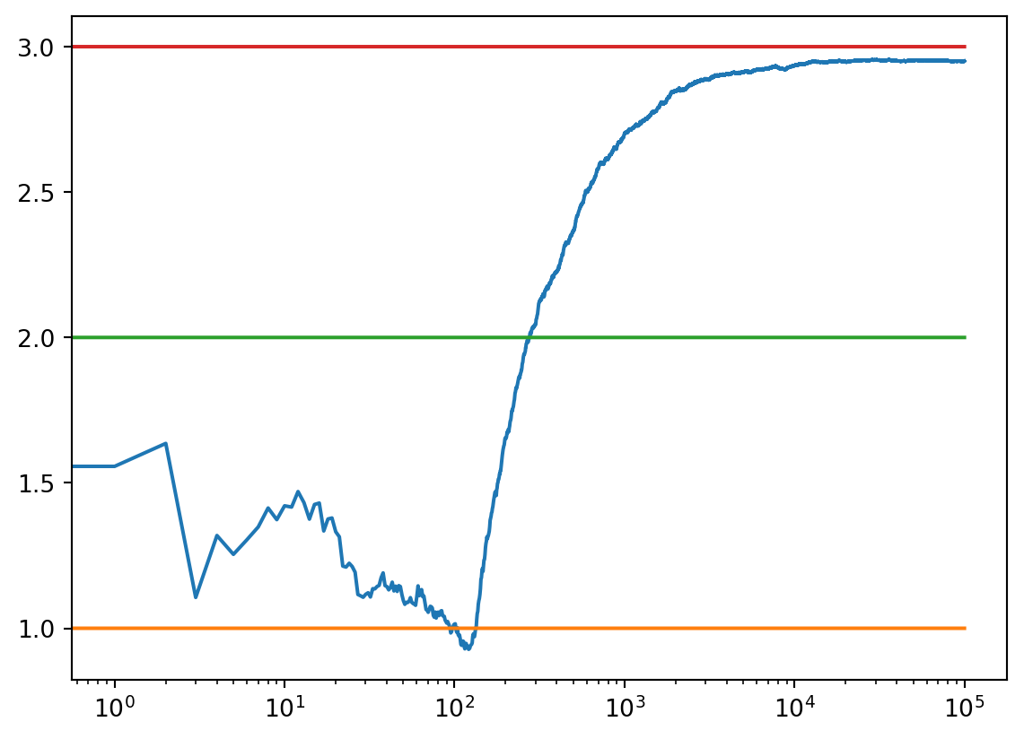
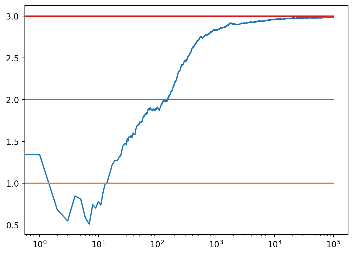
The following is a simple implementation of the Ɛ-greedy algorithm in Python from geeksforgeeks.org
Code
# Import required libraries import numpy as np import matplotlib.pyplot as plt # Define Action class class Actions: def__init__(self, m): self.m = m self.mean =0self.N =0# Choose a random action def choose(self): return np.random.randn() +self.m # Update the action-value estimate def update(self, x): self.N +=1self.mean = (1-1.0/self.N)*self.mean +1.0/self.N * x def run_experiment(m1, m2, m3, eps, N): actions = [Actions(m1), Actions(m2), Actions(m3)] data = np.empty(N) for i inrange(N): # epsilon greedy p = np.random.random() if p < eps: j = np.random.choice(3) else: j = np.argmax([a.mean for a in actions]) x = actions[j].choose() actions[j].update(x) # for the plot data[i] = x cumulative_average = np.cumsum(data) / (np.arange(N) +1) # plot moving average ctr plt.plot(cumulative_average) plt.plot(np.ones(N)*m1) plt.plot(np.ones(N)*m2) plt.plot(np.ones(N)*m3) plt.xscale('log') plt.show() for a in actions: print(a.mean) return cumulative_average
findfont: Font family ['STIXGeneral'] not found. Falling back to DejaVu Sans.
findfont: Font family ['STIXGeneral'] not found. Falling back to DejaVu Sans.
findfont: Font family ['STIXGeneral'] not found. Falling back to DejaVu Sans.
findfont: Font family ['STIXGeneral'] not found. Falling back to DejaVu Sans.
findfont: Font family ['STIXNonUnicode'] not found. Falling back to DejaVu Sans.
findfont: Font family ['STIXNonUnicode'] not found. Falling back to DejaVu Sans.
findfont: Font family ['STIXNonUnicode'] not found. Falling back to DejaVu Sans.
findfont: Font family ['STIXSizeOneSym'] not found. Falling back to DejaVu Sans.
findfont: Font family ['STIXSizeTwoSym'] not found. Falling back to DejaVu Sans.
findfont: Font family ['STIXSizeThreeSym'] not found. Falling back to DejaVu Sans.
findfont: Font family ['STIXSizeFourSym'] not found. Falling back to DejaVu Sans.
findfont: Font family ['STIXSizeFiveSym'] not found. Falling back to DejaVu Sans.
findfont: Font family ['cmtt10'] not found. Falling back to DejaVu Sans.
findfont: Font family ['cmb10'] not found. Falling back to DejaVu Sans.
findfont: Font family ['cmss10'] not found. Falling back to DejaVu Sans.
findfont: Font family ['DejaVu Sans Display'] not found. Falling back to DejaVu Sans.
In the short term we may maximize rewards following the best known course of action. However this may represent a local maximum.
In the long term agents that explore different options and keep uncovering better options until they find the best course of action corresponding to the global maximum.
To get the best of both worlds we need to balance exploration and exploitation ideally using a policy that uses feedback to adapt to its environment.
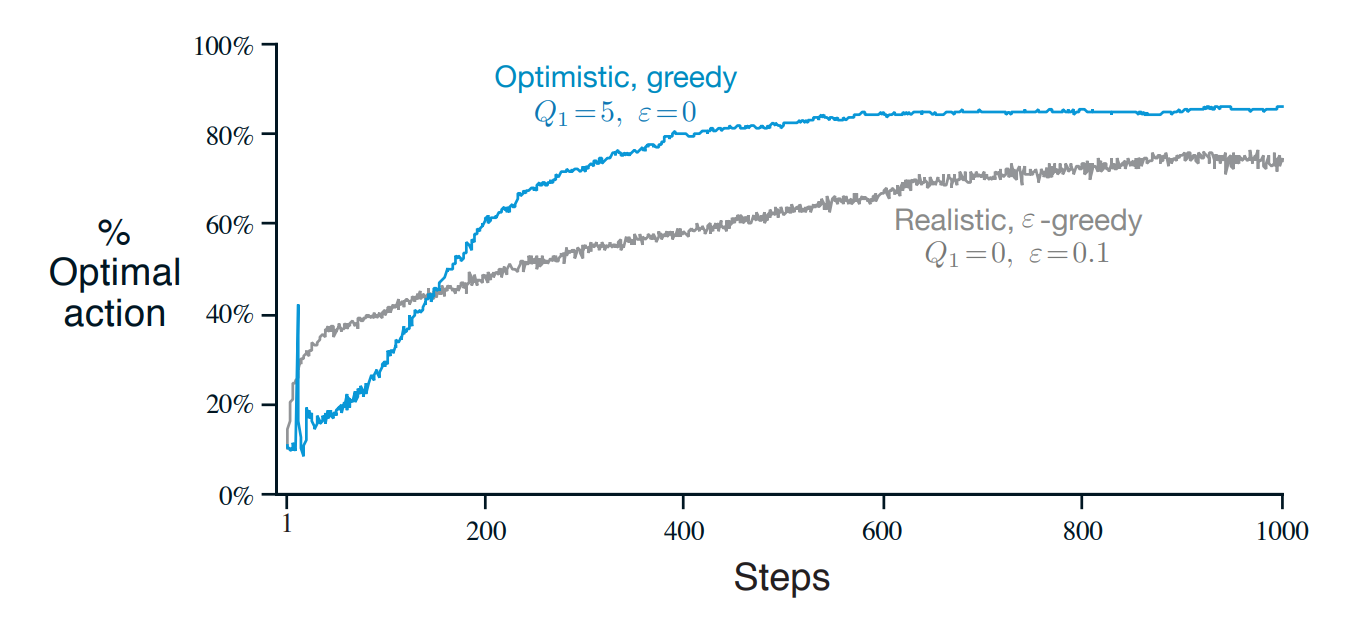
Optimistic initial values
Definition 1 (Optimistic initial values) Setting all initially action values greater than the algorithmically available values in [0,1]
The methods we have discussed are dependent on the initial action-value estimates, Q_1(a). In the language of statistics, we call these methods biased by their initial estimates. For the sample-average methods, the bias disappears once all actions have been selected at least once. For methods with constant \alpha, the bias is permanent, though decreasing over time.
Benefits of optimistic initial values for early exploration
Setting the initial action values to be higher than the true values has the effect of causing various bandit algorithm to try to exploit them - only to find out that most values are not as rewarding as it was led to expect.
What happens is that the algorithm will initially explore more than it would have otherwise. Possibly even trying all the actions at least once.
In the short-term it will perform worse than Ɛ- greedy which tend to exploit. But as more of the state space is explored at least once the algorithm will beat an Ɛ-greedy policy which can take far longer to explore the space and find the optimal options.
The effect of optimistic initial action-value estimates
CautionCriticisms of optimistic initial values
Optimistic initial values only drive early exploration. The agent will stop exploring once this is done.
For a non-stationary problems - this is inadequate.
In a real world problems the maximum reward is an unknown quantity.
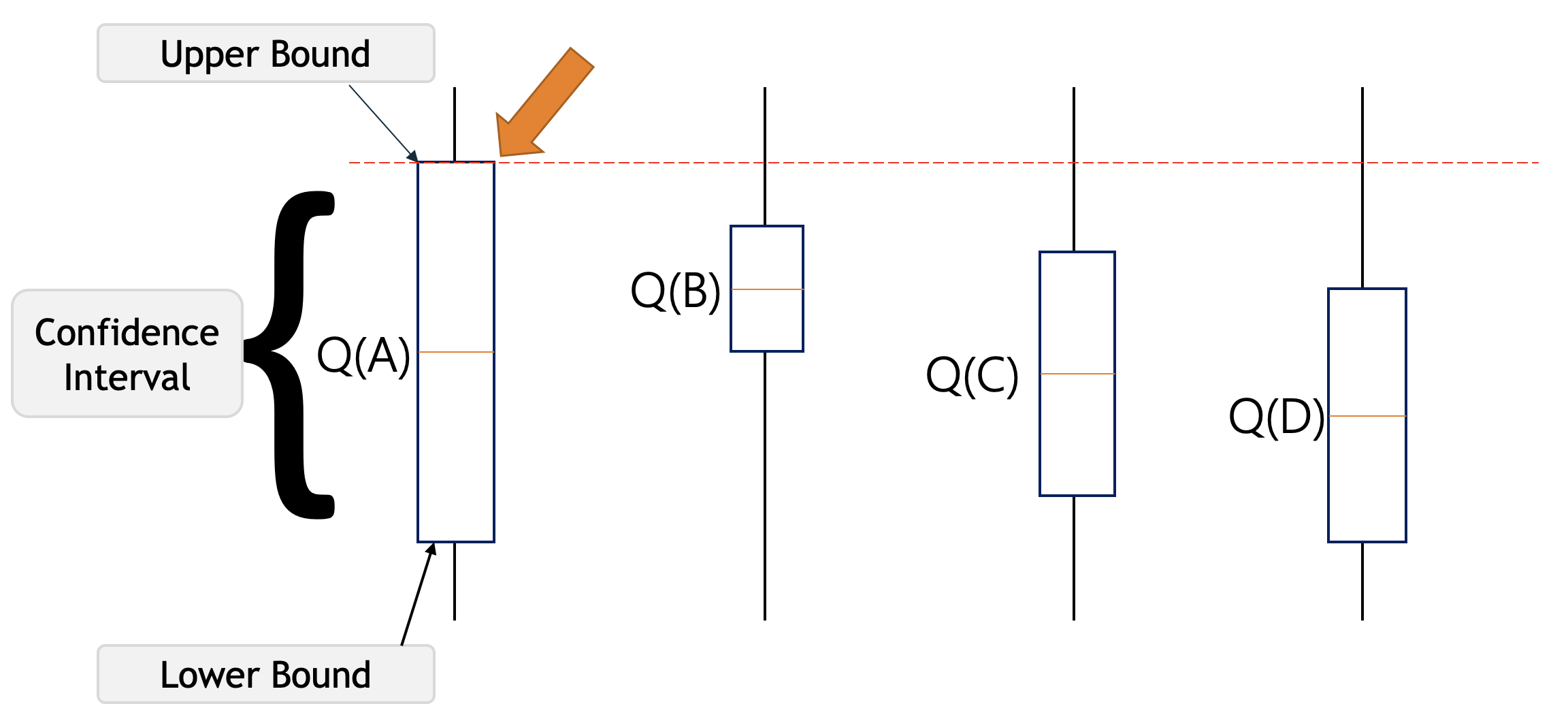
The UCB action selection method
UCB is an acronym for Upper Confidence Bound. The idea behind it is to select the action that has the highest upper confidence bound. This has the advantage over epsilon greedy that it will explore more in the beginning and then exploit more as the algorithm progresses.
c is a constant that determines the degree of exploration
N_t(a) is the number of times action a has been selected prior to time t
UCB intuition
The idea is we the action for which the action value plus the highest possible uncertainty give the highest sum. We are being optimistic in assuming this choice will give the highest reward. In reality any value in the confidence interval could be the true value. Each time we select an action we reduce the uncertainty in the exploration term and we also temper our optimism of the upper confidence bound by the number of times we have selected the action. This means that we will prefer to visit the actions that have not been visited as often.
The main advantage of UCB is that it is more efficient than epsilon greedy in the long run. If we measure the cost of learning in terms of the regret - the difference between the expected reward of the optimal action and the expected reward of the action we choose. UCB has a lower regret than epsilon greedy. The downside is that it is more complex and requires more computation.
Thompson sampling is basically like UCB but taking the Bayesian approach to the bandit problem. We start with a prior distribution over the action values and then update this distribution as we take actions. The action we choose is then sampled from the posterior distribution. This has the advantage that it is more robust to non-stationary problems than UCB. The downside is that it is more computationally expensive.
This is a heuristic to ensure initial exploration of all actions by assuming that untried actions have a high expected reward. We then try to exploit them but end up successively downgrading their expected reward when they do not match our initial optimistic assessment.
The downside to this approach is when the space of action is continuous so we can never get to the benefits of exploration.
from tqdm import tqdmfrom mesa import Model, Agentimport numpy as npclass EpsilonGreedyAgent(Agent):""" This agent implements the epsilon-greedy """def__init__(self, model, num_arms, epsilon=0.1):super().__init__(model)self.num_arms = num_armsself.epsilon = epsilonself.q_values = np.zeros(num_arms) # Initialize Q-value estimatesself.action_counts = np.zeros(num_arms) # Track action countsdef choose_action(self):if np.random.rand() <self.epsilon:# Exploration: Choose random armreturn np.random.randint(0, self.num_arms)else:# Exploitation: Choose arm with highest Q-valuereturn np.argmax(self.q_values)def step(self): chosen_arm =self.choose_action() reward =self.model.get_reward(chosen_arm)assert reward isnotNone, "Reward is not provided by the model"self.action_counts[chosen_arm] +=1 step_size =1/self.action_counts[chosen_arm]self.q_values[chosen_arm] += step_size * (reward -self.q_values[chosen_arm])class TestbedModel(Model):""" This model represents the 10-armed bandit testbed environment. """def__init__(self, num_arms, mean_reward, std_dev,num_agents=1):super().__init__()self.num_agents = num_agentsself.num_arms = num_armsself.mean_reward = mean_rewardself.std_dev = std_devself.env_init()for _ inrange(self.num_agents):self.create_agent(EpsilonGreedyAgent, 0.1)def env_init(self,env_info={}):self.arm_means = np.random.normal(self.mean_reward, self.std_dev, size=self.num_arms)def create_agent(self, agent_class, epsilon):""" Create an RL agent instance with the specified class and parameters. """return agent_class(self, self.num_arms, epsilon)def step(self):self.agents.shuffle_do("step")def get_reward(self, arm_id):return np.random.normal(self.arm_means[arm_id], 1.0)# Example usagemodel = TestbedModel(10, 0, 1) # Create model with 10 armsnum_runs =200# The number of times we run the experimentnum_steps =1000# The number of pulls of each arm the agent takes# Run simulation for multiple stepsfor _ in tqdm(range(num_runs)):for _ inrange(num_steps): model.step() model.step()
Sutton, R. S., and A. G. Barto. 2018. Reinforcement Learning, Second Edition: An Introduction. Adaptive Computation and Machine Learning Series. MIT Press. http://incompleteideas.net/book/RLbook2020.pdf.
.png)