Political Scenario Prediction Using Game theory

A review of (De Mesquita 2011)

De Mesquita, Bruce Bueno. 2011. “A New Model for Predicting Policy Choices: Preliminary Tests.” Conflict Management and Peace Science 28 (1): 65–85. http://www.jstor.org/stable/26275398.

This technical paper is fairly challenging to understand. The main thrust of this work is when conducting an intelligence assessment of some future political scenario, assuming one can identify the main actors their relative influence, their positions and their belief about other players we can use a formal model to assess how they will behave and interpret various outcomes.

Now there are any number of ways this can go bad:

1. we don’t know all the key players
2. we don’t know their stated position
3. we don’t know their influence
4. key players can change due to high leverage low probability events, e.g. 

• the key actor getting assassinated
• the key actor getting indicted and reversing their positions

5. Game theory isn’t the best framework for generating predictions, it’s much better for understanding the mechanics of how drive behavior.

So now that we named the elephants in the room, we can talk about can address the least interesting part of the paper - the fact that the models perform very well when fed with data from expert analysts, assuming that the raw data is accurate.

Prior work by Tatelock outlines the notion of comparing forecasting skill of analysts AKA experts who engage in competition characterizes their abilities. Tatelock call the best Superforcastors suggesting that there is method behind all this madness. A second claim is that formal Models tend to outperform the experts given their raw data. Mesiqua explains that this is due to reduced variance.

My current interest are:

1. how to structure problems so we can analyze them using this approach
2. how to solve this type of game model.
3. how to interpret the results
4. automate data collection
5. try more sophisticated approaches

I suppose that if you get good at structuring the problem then interpretation can be much easier.

In some senses the old model is very simple considering how well it performs. Yet Bayesian games are the kind of games we all played in preschool or at least not to solve them for a perfect Bayesian equilibrium. So there is that inherent mathematical complexity to deal with. If I’m not mistaken the author is bent on reporting his successes without revealing too much about how to reproduce his work. I haven’t review the relevant papers. A second big chunk of this paper deals with the performance of the old model and responding to criticism of his work. So the readers need to decipher as much as they can. However it is not very much motivated. BBdM is an eloquent speaker and an excellent author of several book.

Abstract

A new forecasting model, solved for Bayesian Perfect Equilibria ¹ , is introduced, along with several alternative models, is tested on data from the European Union. The new model, which allows for contingent forecasts and for generating confidence intervals around predictions, outperforms competing models in most tests despite the absence of variance on a critical variable in all but nine cases. The more proximate the political setting of the issues is to the new model’s underlying theory of competitive and potentially coercive politics, the better the new model does relative to other models tested in the European Union context.

¹ surely a sub-perfect equilibrium, to remove pathological solutions?

Summary

Presenting a game theory model in an effort for estimating future states of the world.

The Original Model

old-model

My original forecasting model—the model sometimes referred to as the expected utility model—is quite simple (Bueno de Mesquita, 1984, 1994, 2002). ²

² seems like this section is here to retort to criticism of the old model than motivation

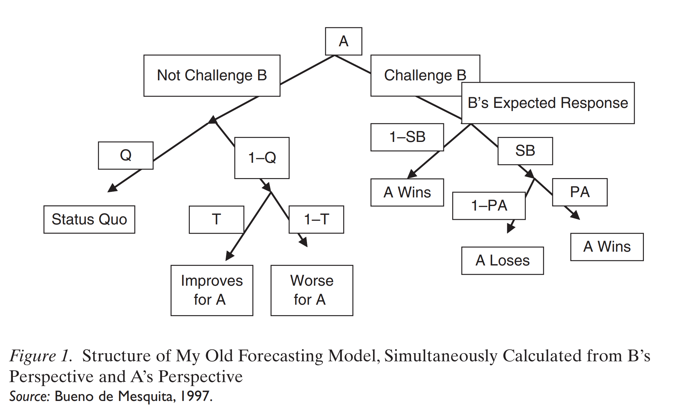
1. player A chooses whether or not to challenge the position of another player B.
2. If the choice is not to challenge then one of three outcomes can arise.

As a consequence of the other dyadic games being played with this player or with other players, the first-mover (player A) believes with probability Q (with Q = 0.5 in the absence of an independent measure of its value) that the status quo will continue and with a 1–Q probability (0.5) it will change. If the status quo vis-à-vis the other player in this model (player B) is expected to change, then how it is expected to change is determined by the spatial location of A and B on a unidimensional issue continuum relative to the location of the status quo or the weighted median voter position on that same continuum. The model assumes that players not only care about issue outcomes but also are concerned about their personal welfare or security. Hence, they are anticipated to move toward the median voter position if they make an uncoerced move. This means that if B lies on the opposite side of the median voter from A, then A anticipates that if B moves (probability = T, fixed here so that T=1.0 under the specified condition), B will move toward the median voter, bringing B closer to the policy outcome A supports. Consequently, A’s welfare will improve without A having to exert any effort. If B lies between the median voter position and A, then A’s welfare worsens (1–T=0) and if A lies between B and the median voter position then A’s welfare improves or worsens with equal probability, depending on how far B is expected to move toward the median voter position. That is, if B moves sufficiently little that it ends up closer to A than it had been, then A’s welfare vis-à-vis B improves; if B moves sufficiently closer to the median voter position that it ends up farther from A than it was before, then A’s welfare declines.

In the old model, if A challenges, then B could either give in to the challenger’s demand (probability = 1–SB) or resist (probability SB) and if B resists then the predicted outcome is a lottery over the demands made by A and B (the position A demands B adopts and B demands A adopts; that is, A’s declared position and B’s declared position) weighted by their relative power (PA = probability A wins) taking into account the support they anticipate from third parties. The same calculation is simultaneously undertaken from the perspective of each member of a dyad so that there is a solution computed for A vs. B and for B vs. A. The fundamental calculations are:

EU|A\ Challenges = (1-S_B)U_{wins} +S_B(P_A)U_{Wins} + S_B(1-P_A)U_{Loses}

EU|A\ Not\ Challenge = Q(U_{StatusQuo}) + (1–Q)[(T)(U_{Improves}) + (1–T)(U_{Worse})]

E^A(U_{AB}) = EU|A\ Challenges – EU|A\ Not\ Challenge

with - S referring to the salience the issue holds for the subscripted player; - P denotes the subscripted player’s subjective probability of winning a challenge; - U’s refer to utilities with the subscripts denoting the utility being referenced.

A estimates these calculations from its own perspective and also approximates these computations from B’s perspective. Likewise, B calculates its own expected utility and forms a view of how A perceives the values in these calculations. Thus there are four calculations for each pair of players:

1. E^A(U_{AB})
2. E^A(U_{BA})
3. E^B (U_{AB})
4. E^B (U_{BA})

The details behind the operationalization of these expressions are available elsewhere (Bueno de Mesquita, 1994, 1999). The variables that enter into the construction of the model’s operationalization are:

1. Each player’s current stated or inferred negotiating position (rather than its ideal point);
2. Salience, which measures the willingness to attend to the issue when it comes up; that is, the issue’s priority for the player; and
3. Potential influence; that is, the potential each player has to persuade others of its point of view if everyone tried as hard as they could.

Surprisingly, given how simple this model is, it is reported by independent auditors to have proven accurate in real forecasting situations, about 90% of the time in more than 1,700 cases according to Feder’s evaluations within the CIA context (Feder, 1995, 2002; Ray and Russett, 1996). Both the experts and the model were pointing in the right direction 90% of the time, but the model greatly outperformed the experts in precision (lower error variance) according to Feder. Feder also notes that in the cases he examined, when the Policon model and the experts disagreed, the model proved right and not the experts who were the only source of data inputs for the model.

Tetlock (2006) has demonstrated that experts are not especially good at foreseeing future developments. Tetlock and I agree that the appropriate standard of evaluation is against other transparent methodologies in a tournament of models all asked to address the same questions or problem. In fact, I and others have begun the process of subjecting policy forecasting models to just such tests in the context of European Union decision making (Bueno de Mesquita and Stokman, 1994; Thomson et al., 2006; Schneider et al., 2010). This article is intended to add to that body of comparative model testing. And, of course, Tetlock’s damning critique of experts notwithstanding, we should not lose sight of the fact that most government and business analyses as well as many government and business decisions are made by experts. However flawed experts are as prognosticators, improving on their performance is also an important benchmark for any method.

Thomson et al. (2006) tested the expected utility model against the European Union data that are used here. They found that it did not do nearly as well in that cooperative, non-coercive environment as it did in the forecasts on which Feder reports. Achen (2006), as part of Thomson et al.’s project, in fact found that the mean of European Union member positions weighted by their influence and salience did as well or better than any of the more complex models examined by Thomson et al. (2006). I will return to this point later when we examine the goodness of fit of the various approaches tested by Thomson et al. (2006) and the new model I am introducing here.

new model

Structure of the New Model

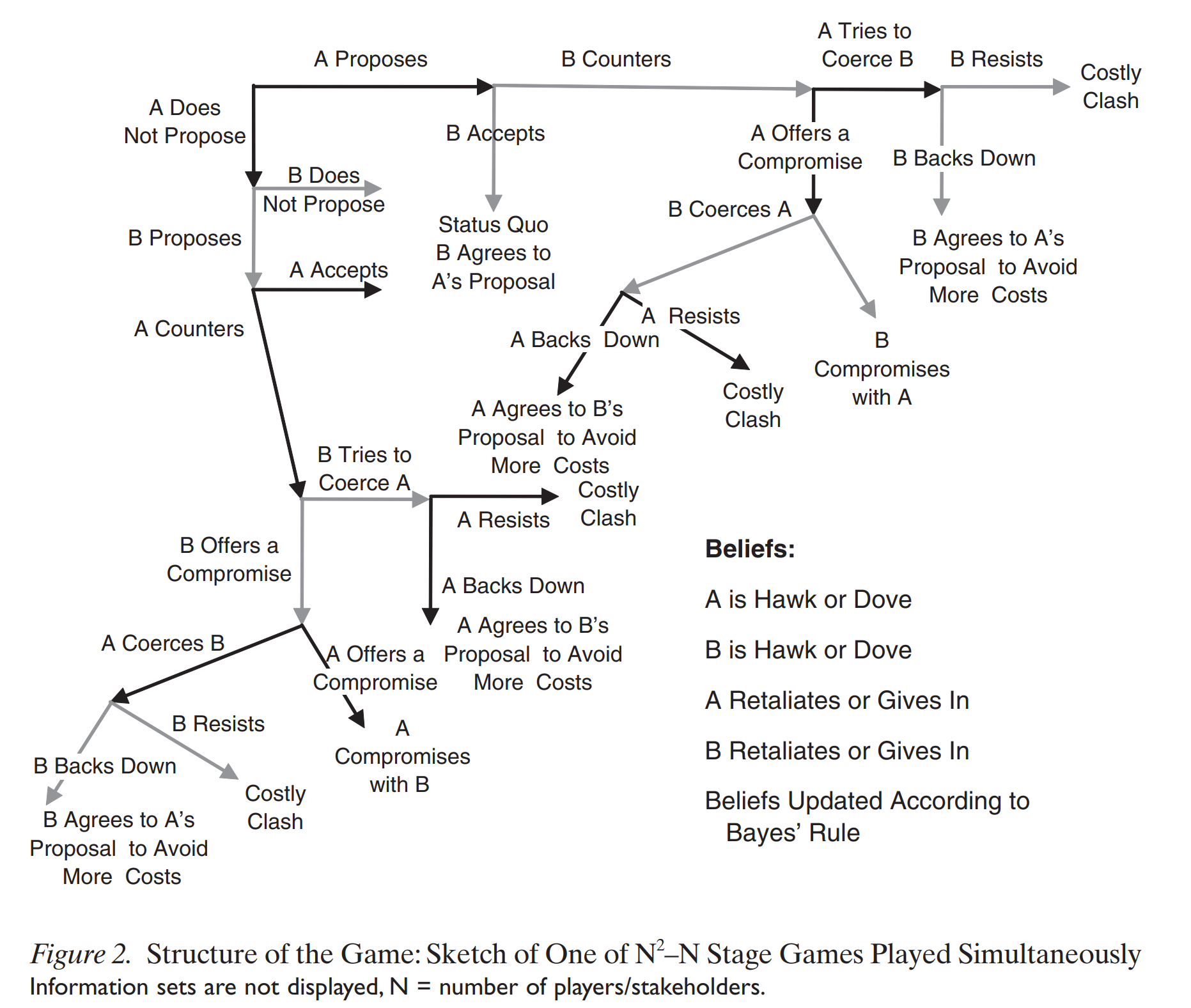
The new model’s structure is much more complex than the expected utility model and so it will be important for it to outperform that model meaningfully to justify its greater computational complexity. Inputs are, in contrast, only modestly more complicated or demanding although what is done with them is radically different.

Each player is uncertain whether the other player is a hawk or a dove and whether the other player is pacific or retaliatory. By hawk I mean a player who prefers to try to coerce a rival to give in to the hawk’s demands even if this means imposing (and enduring) costs rather than compromising on the policy outcome. A dove prefers to compromise rather than engage in costly coercion to get the rival to give in. A retaliatory player prefers to defend itself (potentially at high costs), rather than allow itself to be bullied into giving in to the rival, while a pacific player prefers to give in when coerced in order to avoid further costs associated with self-defense. The priors on types are set at 0.5 at the game’s outset and are updated according to Bayes’ Rule. This element is absent in Bueno de Mesquita and Lalman (1992). In fact, the model here is an iterated, generalized version of their model, integrating results across N(N–1) player dyads, introducing a range of uncertainties and an indeterminate number of iterations as well as many other features as discussed below. Of course, uncertainty is not and cannot be limited to information about player types when designing an applied model. We must also be concerned that there is uncertainty in the estimates of values on input variables whether the data are derived, as in the tests here, from experts or, as in cases reported on in the final two

there are 4 type of players: <[hawk|dove],[pacific,retalitory]>